Latest Posts
Tips for preparing for an Oxbridge undergraduate maths interview
First published September 12, 2024From my experience as an interviewer, some advice for students preparing for an undergraduate admissions interview in maths at Oxford or Cambridge.
Over time, I intend to occasionally update this post with new resources and suggestions.
What’s the structure of the interview?
Most interviews are about 30 minutes in length. The contents of the interview will be almost entirely mathematical, with maybe some softer questions at the start to serve as a warm-up.
From the point of view of the college, the interview is a chance for them to see first-hand how you think when faced with a challenging and unseen problem. For the most part, the interviewers will sit back and observe your working, but will occasionally step in and provide suggestions if they feel it could be helpful to you.
Since the pandemic, almost all interviews at Oxford are currently held online. At Cambridge, some colleges are once again holding some interviews in-person. See here for details.
Where to find interview practice questions?
Finding practice questions is probably one of the trickiest parts of preparing for an interview. There are many websites out there which present huge lists of ‘practice questions’. Some of these can be helpful, though my opinion is that many of these practice questions are, quite frankly, a bit rubbish. I suggest also looking at the following resources.
1. MAT papers
Questions from the Maths Admissions Test (MAT) are a good source of practice. If there are any past papers questions which you have not seen before, then take the time to imagine they’re interview questions and answer them accordingly.
MAT past papers are available here.
2. TMUA papers
Similar to the MAT, the TMUA can also serve as a good source of practice.
Continue reading...A brief history of three-dimensional manifolds
First published November 24, 2022We give a broad-brush account of some milestones in the theory of 3-dimensional manifolds, particularly the Poincaré Conjecture and its proof. We also discuss Thurston’s Geometrisation Programme.
This post is adapted from a short project I completed last year. Do get in touch with any corrections.
1. The Beginning - from Poincaré to Dehn
The theory of three-dimensional manifolds has been a topic of great interest for well over a century, and we begin our account with the work of Henri Poincaré.
In [25], Poincaré introduces the notion of the fundamental group of a space. He believed that such a tool could lead to a more sophisticated classification of topological spaces than had existed before. In a later work [26], Poincaré raises the following question, which inspired generations of mathematicians.
Est-il possible qu le groupe fondamental de \(V\) se réduise à la substitution identique, et que pourtant \(V\) ne soit pas simplement connexe?
With modern terminology, this translates to the question “Is it possible for the fundamental group of [the 3-manifold] \(V\) to be trivial, but that \(V\) is not homeomorphic to the 3-sphere?” This question came to be known as the Poincaré conjecture. As a small aside, it is worth pointing out that the above literally translates to “Is it possible that the fundamental group of \(V\) consists of only the identity, and that yet \(V\) is not simply connected?” This is obviously false under modern definitions. Indeed the definition of simply connected has changed over time, and this is an interesting example of how terminology can evolve.
The work of Poincaré was of incredible importance, due to the new ideas it put forward. However, Chandler and Magnus [5] remark that much of Poincaré’s work is difficult to read and sometimes imprecise, as much of the work fails to “separate intuition from proof”. Many of these ideas were reformulated in a rigorous fashion by Tietze, in his landmark work [36]. This article is based on the work of Poincaré, and re-introduces the concept of a manifold (defined as a cell complex), as well as the fundamental group of such a space. Tietze goes on to prove many foundational results which set the stage for algebraic topology, such as the fact that homeomorphic manifolds have isomorphic fundamental groups. Considering 3-manifolds in particular, Tietze summarises his findings with the following quote:
[…] the fundamental group of an orientable closed three-dimensional manifold contributes more to its characterisation than all the presently known topological invariants taken together.
The above only consolidates the importance of the Poincaré conjecture.
Indeed, Poincaré’s work inspired that of many more mathematicians, including that of Max Dehn. In [7], Dehn builds upon the work of Tietze and Poincaré to make further progress in studying and classifying 3-manifolds based on their fundamental groups. This work then inspired much of Dehn’s contributions to group theory, leading to a later paper [8] formulating his three famous fundamental problems: the word, conjugacy, and isomorphism problems.
There is much more that could be said about this period, but it is beyond the scope of this report. We thus point the interested reader to [5] for a detailed account of this period and the subsequent emergence of combinatorial (later, geometric) group theory.
2. The Mid-20th Century - from Kneser to Johannson
We now jump ahead in time, and consider a selection of important results from the middle of the twentieth century. We begin with a classical decomposition theorem, for the statement of which we will need the following definition.
Definition 2.1. We say that a 3-manifold \(M\) is prime if \(M\) cannot be expressed as a connected sum \(M \cong M_1 \# M_2\), where neither \(M_i\) is \(S^3\).
Continue reading...Measuring angles within arbitrary metric spaces
First published October 02, 2020We will generalise the concept of angles in Euclidean space to any arbitrary metric space, via Alexandrov (upper) angles.
A familiarity with metric spaces shall be assumed for obvious reasons, as well as a passing familiarity with inner product spaces.
1. Introduction and Preliminaries
Before we can generalise we must agree on a definition: what is an angle? Wikipedia gives the following answer to this question.
In plane geometry, an ‘angle’ is the figure formed by two rays, called the sides of the angle, sharing a common endpoint, called the vertex of the angle. […] ‘Angle’ is also used to designate the measure of an angle or of a rotation.
Defining an angle as a figure will not lead to any interesting mathematics, so for the purposes of this post we shall identify an angle with its size. More formally, we will think of an (interior) angle in the Euclidean plane \(\mathbb R^2\) as a function \(\angle\) mapping two straight lines which share an endpoint to a real number \(\alpha \in [0,\pi]\). Clearly then, if we wish to generalise this idea of “angles” to a generic metric space, we must first generalise what we mean by a “straight line”. In metric geometry, we typically achieve this by define a “straight line” as an isometric embedding of some closed interval. This embedding is known as a geodesic, and is defined precisely as follows.
Definition 1.1. (Geodesics) Let \((X,d)\) be a metric space. A map \(\varphi : [a,b] \to X\) is called a geodesic if it is an isometric embedding, i.e. if for all \(x,y \in [a,b]\), we have
\[d(\varphi(x), \varphi(y)) = | x - y |.\]We say \(\varphi\) issues from \(\varphi(a)\). We say that \(\varphi\) connects \(\varphi(a)\) and \(\varphi(b)\), and a space where any two points may be connected by a geodesic is a geodesic space. If this geodesic is always unique (i.e. precisely one geodesic connects any two points in a space), the space is said to be uniquely geodesic.
We similarly we refer to an isometric embedding \(\psi : [c,\infty) \to X\) as a geodesic ray. The image of a geodesic or geodesic ray is called a geodesic segment. We may sometimes denote a geodesic segment between two points \(x\) and \(y\) in space by \([a,b]\).
Our goal here is to generalise the Euclidean definition of an angle between two geodesics, typically defined using the classical law of cosines such that it may be applied to an arbitrary metric space. This will take the form of a function \(\angle\) which will take as input two geodesics (or geodesic rays) issuing from the same point and output a real number in the required range.
Remark. At this point, we may note that an arbitrary metric space need not contain any geodesic segments. One may now be tempted to point out that the title of this post is thus an exaggeration and the upcoming definition cannot possibly apply to all metric spaces. I would retort however that for a metric space \(X\), the statement “we can measure the angle between any two geodesics in \(X\) with a shared endpoint” holds even in the case that no such geodesics exist in \(X\), for the same reason that “every element of the empty set is puce-coloured” holds.
Before we get to our key definitions, some notational and terminological remarks. The Euclidean norm will be denoted by \(\| \cdot \|_2\). Secondly, when we refer to a vector space within this post, we will be speaking specifically about real vector spaces - i.e. vector spaces over the field \(\mathbb R\).
2. Definitions
The overall idea of this generalisation will be to choose a point on each geodesic, and consider the triangle formed by these points and the initial point. We then observe the behaviour of this triangle as these points move arbitrarily close to the initial point, and in taking the limit we will hopefully find our generalisation. Of course to make any sense of the “triangle” formed in our metric space between any three points, we need some way to make a direct comparison to a similar Euclidean shape. This is where the idea of a comparison triangle comes in, and indeed we have our first definition.
Definition 2.1. (Comparison triangles) Let \(X\) be a metric space, and let \(x,y,z \in X\) be points. We define a comparison triangle for the triple \((x,y,z)\) as the triangle in \(\mathbb R^2\) with vertices \(\bar x, \bar y, \bar z\), and side-lengths such that
\[\begin{align} d(x,y) &= \|\bar x - \bar y\|_2, \\ d(x,z) &= \| \bar x - \bar z\|_2, \\ d(y,z) &= \|\bar y - \bar z\|_2. \end{align}\]Note that this triangle is unique up to isometry. Denote this triangle \(\overline \Delta (x,y,z)\). The comparison angle of \(x\) and \(y\) at \(z\), denoted \(\overline \angle_z (x,y)\), is defined as the interior angle of \(\overline \Delta (x,y,z)\) at \(\bar z\).
Remark. Note that comparison triangles are sometimes called model triangles by some authors.
Informally, what we are doing here is simply taking three points in our metric space, measuring the distances between them in this space and constructing a Euclidean triangle with these distances as the side lengths. The triangle inequality within the aforementioned metric space guarantees that this will always be possible given any choice of points. Using this technique, we may compare figures in our metric space with similar figures in the plane. This idea then leads us to the main definition of this post.
Definition 2.2. (Alexandrov angles) Let \(X\) be a metric space, and let \(\varphi : [0,r] \to X\), \(\psi : [0,s] \to X\) be geodesics such that \(\psi(0) = \varphi(0)\). The Alexandrov angle between \(\varphi\) and \(\psi\) is defined as
\[\angle(\varphi, \psi) := \lim_{\varepsilon \to 0} \sup_{0 < t,t' < \varepsilon} \overline \angle _{\varphi(0)} (\varphi(t) ,\psi(t')).\]If the limit
\[\lim_{(t,t') \to^+ (0,0)} \overline \angle _{\varphi(0)} (\varphi(t) ,\psi(t'))\]exists, we say that this angle exists in the strict sense.
Note that these angles will always exist, since \(\overline \angle _{\varphi(0)} (\varphi(t) ,\psi(t'))\) must lie in \([0,\pi]\) and thus the supremum is necessarily finite (and decreasing as \(\varepsilon \to 0\)). However they certainly need not exist in the strict sense, and we shall see some important examples of this shortly.
Intuitively, one can imagine that we choose two points - one on each geodesic, and consider the comparison triangle of these points and the issue point. We then slide these two points towards the issue point and see how the comparison angle changes.
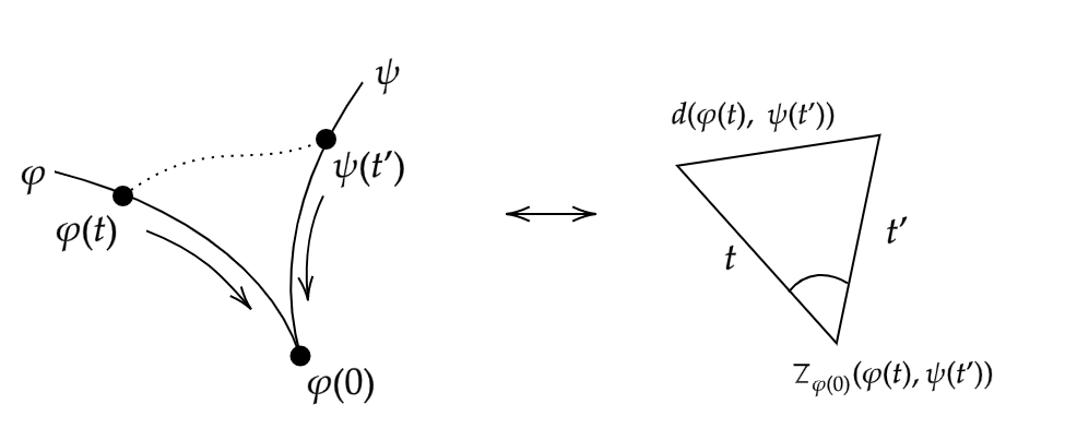
[Click the image for a larger version]
As our points approach the issue point, we will see this comparison angle approach some value.
Continue reading...Hilbert's hotel, but the guests are mere mortals
First published July 26, 2020We will consider a variation of Hilbert’s hotel, within which guests may not be relocated too far from their current room.
This post will be hopefully more accessible than other topics on this site, and should require no more than some basic set theory to comprehend. The contents of this post aren’t meant to be too thought provoking, as the point being made is quite moot. My aim is to demonstrate the (in my opinion) relatively nice combinatorial argument which falls out of this toy problem.
Edit, 26/7/2020: A small translation error has been corrected.
1. Introduction
Hilbert’s Paradox of the Grand Hotel is a relatively famous mathematical thought experiment. It was introduced by David Hilbert in 1924 during a lecture entitled ‘About the Infinite’ [1, p. 730] (translated from the German ‘Über das Unendliche’). Hilbert’s goal in this demonstration was to show how when dealing with infinite sets, the idea that the “the part is smaller than the whole” no longer applies. In other words, the statements “the hotel is full” and “the hotel cannot accommodate any more guests” are not necessarily equivalent if we allow an infinite number of rooms. Hilbert gives the following explanation for how one can free up a room in an infinite hotel with no vacancies.
We now assume that the hotel should have an infinite number of numbered rooms 1, 2, 3, 4, 5 … in which one guest lives. As soon as a new guest arrives, the landlord only needs to arrange for each of the old guests to move into the room with the number higher by 1, and room 1 is free for the newcomer.
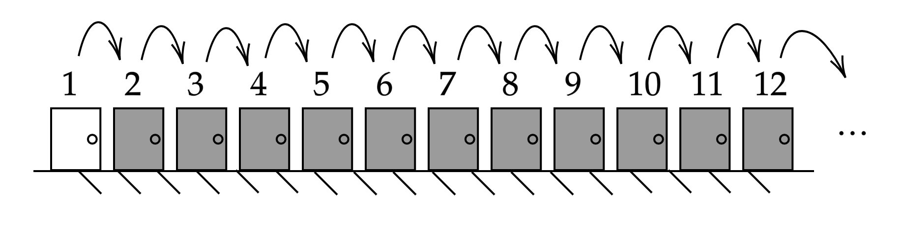
[Click the image for a larger version]
Indeed this can be adjusted to allow for any arbitrary number of new guests. For any natural number \(c\), we can accommodate an extra \(c\) by asking every current guest to move from their current room \(n\) to the room \(n+c\). Upon doing this, the rooms numbered 1 to \(c\) shall become available. Hilbert then goes on to demonstrate that we can extend this to even allowing an infinite number of new guests in our already full hotel.
Yes, even for an infinite number of new guests, it is possible to make room. For example, have each of the old guests who originally held the room with the number \(n\), now move into the one with the number \(2n\), whereupon the infinite number of rooms with odd numbers become available for the new guests.
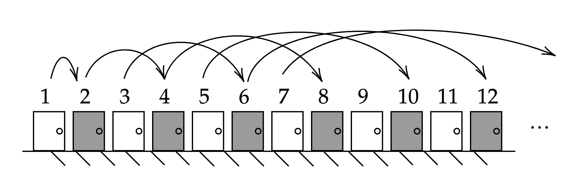
[Click the image for a larger version]
This fact is somewhat remarkable and can seem rather counterintuitive upon first viewing. If we imagine ourselves standing in this hotel’s fictional foyer, the image of a corridor stretching off to infinity is sure to be a daunting one, and trying to make any kind of practical considerations within this setting is surely a fool’s errand. Alas that is exactly what the rest of this post shall try to do.
Suppose that we have our own grand hotel, and every room is currently occupied by a guest with a finite lifespan. We receive word that an infinitely long coach of tourists will be arriving shortly, and are asked to accommodate as many guests as possible. To accomplish this we may move guests between rooms as in the previous case, but with the catch that our current guests must arrive at their new room before their timely demise.
Continue reading...My Oxford postgrad interview: applying for the MFoCS MSc
First published June 21, 2020Here I will summarise my experiences in applying for the Oxford MFoCS, including some tips on how I made my application as competitive as possible.
I don’t intend for this to be a definitive guide to the application process, as I could never claim that my application was perfect. However, I do know that when I was applying I found it difficult to find people openly discussing their own experiences with the application process (especially for this programme which features a relatively small cohort of ~17 people per year). Thus, if just one person in future years finds this post useful when writing their own application, then this summary was worth writing.
1. Introduction
If you are reading this, then I will presume that you would like to apply for the MFoCS at Oxford (or another related programme) and are seeking advice. I will briefly summarise the programme for the less-informed reader, to give context to the rest of this post.
The Oxford MFoCS is the University’s MSc in Mathematics and Foundations of Computer Science. It is a taught programme which runs for 12 months, beginning in Michaelmas term and running into the Summer. The programme is assessed by 5+ mini-projects (extended essays) and a dissertation in the Summer term. Regarding the contents of the course, I will quote the University directly.
The [MFoCS], run jointly by the Mathematical Institute and the Department of Computer Science, focuses on the interface between pure mathematics and theoretical computer science. The mathematical side concentrates on areas where computers are used, or which are relevant to computer science, namely algebra, general topology, number theory, combinatorics and logic. Examples from the computing side include computational complexity, concurrency, and quantum computing.
This programme is a natural fit to anybody coming from a mathematics degree, with any level of interest in the mathematics behind computer science. In this post, I will summarise some key points from my academic CV, statement of purpose, and finally the interview. I will also talk a bit on what followed, hopefully giving some clues to how long the admissions process may take.
Though a very important part of the application process, I will not discuss referees here. An application requires three referees, with at least two being academic in nature (all three of mine were academic). Your referees should be people who can speak confidently about your ability. Other than that, your choice of referees will vary greatly depending on your own prior experience/networking, and there is nothing I can say here to really advise on this.
2. My Academic CV
This was probably the first thing I finished working on during my application. I do not believe that too much weight is placed on the CV, and so I would suggest not spending too much time on this. The official guidance states the following.
A CV/résumé is compulsory for all applications. Most applicants choose to submit a document of one to two pages highlighting their academic achievements and any relevant professional experience.
That being said, my CV was split into five sections across two pages, namely Education, Relevant Employment, Writings, Technical Skills, and Other Awards. These headings are mostly self-explanatory, and the key point to take away is to keep things relevant. Any education will of course be relevant, but employment should be restricted to research, teaching, and anything else which the department might view as appropriate (something related to mathematics and/or computer science would fit this mould).
Continue reading...A simple annual budget template for Google sheets
First published June 06, 2020A template for an annual budget spreadsheet, which tracks one’s spending on a weekly basis.
This budget allows you to input your expected incomes and expenditures for the year ahead, and forecast your balances through the next 12 months. This sheet is especially suited to students, allowing you to know in advance if you’re heading towards your overdraft (or beyond) later in the year.
The template can be found here. This link will lead to a prompt to copy the file, following which the sheet will most likely be available within your ‘My Drive’ folder. The rest of this post will be a brief summary of the functionality available. One will note that there is two different templates – one with investments and one without. These are mostly identical but with some small additions in the former to allow the user to track an investment portfolio as well. This guide will focus on the latter, with an addendum on the former.
1. Overview
First things first, only cells with red font should be editted by the user, and any others left to be automatically filled in. This sheet tracks two balances for the user - a main spending account and a savings account. All spending and income is assumed to be coming in and out of the main account, with the savings account remaining untouched apart from the occasional deposit or withdrawel. The sheet is split vertically into four sections. They are PLANNED, RECORDED, PROJECTED, and MISC.
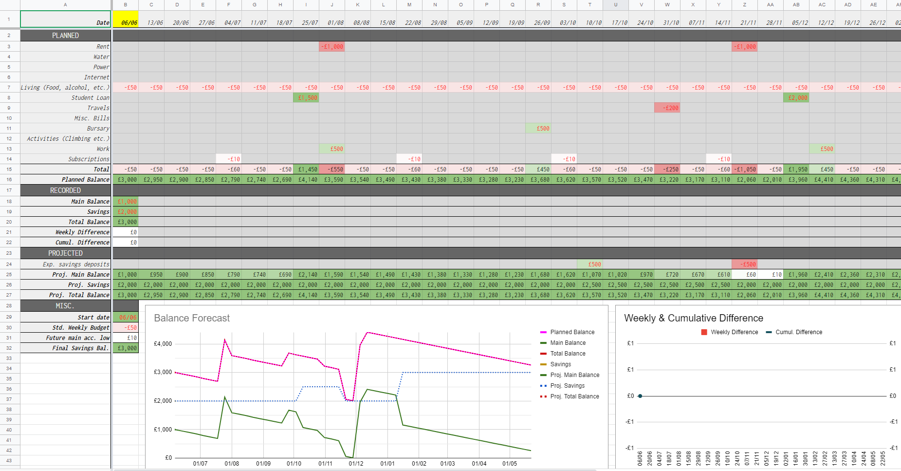
[Click the image for a larger version]
Each column of the sheet represents a week, with the date at the top being the first day of that week. Choose your start date in the bottom-left corner under MISC. and the rest of the year will be filled in. The current week will be highlighted in yellow for visibility. We will now take a more in-depth look at the first three of these sections.
Continue reading...A finitely-generated group that is not finitely presentable
First published November 06, 2019In this post we will work towards an example of a finitely generated group that cannot be expressed by any finite presentation.
For the sake of brevity, I will assume a working knowledge of combinatorial group theory and group presentations, however an informal exposition will be provided in Section 1.
1. Background
Very briefly we shall restate some important definitions and results regarding group presentations with the goal of building up to our main question, the reader who is familiar with such notions can safely skip this section. We will be roughly following the definitions laid out by Magnus in [1]. Combinatorial Group Theory is the study of defining groups with a set of generators, and another set of words in these generators known as relators. More formally, we have the following definitions.
Definition 1.1. (Words) Let X be a set of n symbols and for any symbol \(x\) in X, define its formal inverse as a new symbol \(x^{-1}\). Similarly, the inverse of a symbol \(x^{-1}\) is defined as just \((x^{-1})^{-1} = x\). Let X* be the set of words in these symbols and their inverses (including the empty word, denoted 1), where a word is a finite sequence of symbols. Furthermore, define the formal inverse of a word w in X* as
\[w^{-1} = (x_1 x_2 \ldots x_n)^{-1} = x_n^{-1} \ldots x_2^{-1} x_1^{-1}\]where each \(x_i\) is either an element of X or the inverse of one. Given two words w and v, we define their juxtaposition wv as concatenation in the obvious sense. A word v is a subword of another word w if it itself appears as a contiguous block within w. We may parameterise a word \(w(x,y,z \ldots)\) or \(w(X)\) to denote the set of symbols appearing in w.
Definition 1.2. (Group presentations) Let X be a set of symbols, then a presentation is a pair \(\langle X ; R \rangle\) where R is some subset of X*. Elements of X are known as generators, and elements of R are known as relators.
We say two words w and v in X* are equivalent if v can be obtained from w by a finite sequence of the following operations.
-
Insertion of any element of R or its inverse, or a string of the form \(xx^{-1}\) or \(x^{-1}x\) where \(x \in X\), in between any two consecutive symbols, or at the beginning or end of the w.
-
Deletion of any element of R or its inverse, or a string of the form \(xx^{-1}\) or \(x^{-1}x\) where \(x \in X\), if it appears as a subword of w.
This forms an equivalence relation on X* (we will not check this here), and it is clear that any relator lies within the class of the empty word. Define the following operation on the set of equivalence classes,
\[[w] \cdot [v] = [wv],\]where v, w are elements of X*, and indeed this forms a group with the class of the empty word as the identity, and the obvious inverses (which is another fact we will not check). Given some presentation P, denote its equivalence class group \(\overline{P}\). One can think of relators as equations, where if the word R is a relator, then we stipulate \(R = 1\) within our group. We may sometimes abuse notation and write relations \(X = Y\) instead of relators in our group presentations, but it isn’t hard to see that this doesn’t change anything (every relation can be re-expressed as a relator). If a relation holds in a group given by a presentation, then this relation is said to be derivable from the given relations.
We have that every presentation defines a group, and in fact it is also true that every group is defined by some presentation. More precisely we have the following theorem.
Theorem 1.1. (Equivalence of groups and presentations) Let G be some group, then there exists a presentation P such that G is isomorphic to \(\overline{P}\). Furthermore, every presentation defines a group in the above way.
So our notions of presentations and groups are indeed equivalent, though a given group may have many different presentations. A group G is called finitely generated if there exists a presentation for G with a finite set of generators, and similarly a group is called finitely presentable if there exist a presentation for G with both a finite set of generators and relators. The goal of this post is to work towards an example of a group which is finitely generated but not finitely presentable, and demonstrate that these two conditions are indeed very different.
2. Redundant Relators
We shall consider a result presented by B. H. Neumann, in his 1937 paper Some remarks on infinite groups [2]. This result about finitely presentable groups will be used in Section 3 to argue that our construction cannot be finitely presentable, by contradiction.
Theorem 2.1. Let G be a group defined by the finite presentation \(\langle x_1 \ldots x_n ; R_1, \ldots R_m \rangle\), and some suppose that \(Y = \{y_1, \ldots y_l\}\) is another finite generating set of G. Then, G can be defined with finitely many relators in Y.
Proof. Write \(X=\{ x_1 \ldots x_n \}\), we consider the following sequence of transformations. First, we write each \(x_i\) in terms of Y, and vice versa, as both X and Y generate G. That is,
\[x_i = X_i(Y), \ \ y_j = Y_j(X),\] Continue reading...Quantum search for the everyday linear algebraist
First published August 11, 2019I present a brief introduction to quantum computation, and particularly Grover’s search algorithm, written for the average linear algebraist.
I have written this piece with the goal of not requiring any prior knowledge of quantum computation - but will be assuming a good working knowledge of linear algebra and complex vector spaces. I also assume knowledge of Big-O notation though this is fairly self-explanatory in context.
1. Introduction
Consider the problem of finding a particular marked item in an completely unsorted list. With no structure or order to abuse, the only option we are left with is essentially checking each element of the list one-by-one, hoping we come across our marked entry at some point in the near future. It’s easy to argue that in a list of N items, we would need to check an expected number of N/2 items before we come across our item, and N-1 to find it every time with certainty.
Of course in a sorted list, we could do much better using techniques like binary-search to improve our number of queries to O(log N). Sadly this is of no use to us here, and if we wish to gain any kind of speed-up to this process we will need to leave the realms of classical computation.
In 1996, Lov Grover presented his revolutionary quantum search algorithm [1], which makes use of quantum mechanics to find the marked item with high probability, using only \(O(\sqrt N)\) queries. This is quite the result. For some concreteness consider an unsorted list of 1,000,000 elements. Classically, to find our marked item we would have to check pretty much every element in the list, in the worst case. However, Grover’s algorithm would find the marked item with roughly 800 queries to this list - a very dramatic improvement. There is some subtlety as to what we mean by a query in the quantum case, but we will discuss this in section 3.
2. Quantum Computation
In this section we will provide a brief description of quantum computation in general, for some context to the algorithm. First, lets consider classical, deterministic computation. We will have a system that starts in some initial state - say a binary register set to 00…0 - and our algorithm will change this state to another state. The system will only ever be in one state at any given moment but may cycle through plenty of different states over time while the algorithm computes. Every choice the algorithm makes is completely deterministic, and so our algorithm is essentially a function mapping from states to states. However, it need not be this way.
Grover [1] describes quantum computation with an analogy to probabilistic algorithms. Consider an algorithm that flips a coin at some point(s), and decides what to do next based on the result(s). We can then model the outcome of the algorithm (as well as all intermediate steps) with a probability distribution of possible states that the system could be in. In particular, the state of the system could be described by a vector \((p_1,\ldots,p_N)\) where each component contains the probability of being in a particular state at that point in time (note that we can think of the standard basis vectors \((1,0,\ldots,0)\) etc. as being our classic “deterministic” states where if the algorithm terminated there, we would know the precise outcome with certainty). Steps of the algorithm can be thought of as multiplying these vectors by some kind of transition matrix. Within this model it should be clear that we are restricted to the conditions that at any point the components of this probability vector must sum to 1 (else we haven’t got a correct distribution) and our transition matrices mustn’t affect this property. After a probabilistic algorithm runs it will output some result which is probably what you want, given that you designed your algorithm well.
Quantum computation is a bit like this, though arguably more exciting. Instead of probabilities, we deal with amplitudes. These amplitudes are complex numbers and a vector of these amplitudes is called a superposition of possible states the system could be in. One can measure a quantum superposition, and this will cause it to collapse into one of these states with probability equal to the square of the modulus of its amplitude. Again, from this model its straightforward to see that since we are dealing with probabilities, we are subject to the normalisation condition where given a superposition \((\alpha_1, \ldots , \alpha_N )\), we must have
\[\sum_{i=1}^N | \alpha_i |^2 = 1\]and our transition matrices must preserve this property. It can be checked that the only matrices that preserve this property are unitary transformations, though the details of this I am declaring beyond the scope of this post. Thus a quantum computation is essentially a chain of some number of unitary operations acting on our state space, which is essentially \(\mathbb{C}^N\).
Continue reading...Modular machines and their equivalence to Turing machines
First published June 18, 2019Modular machines are a lesser-known class of automata, which act upon \(\mathbb{N}^2\) and are actually capable of simulating any Turing Machine - a fact which we will prove here.
The purpose of this post is to provide solid, self-contained introduction to these machines, which I found was surprisingly hard to find. My goal has been to collate and expand upon the relevant descriptions given by Aanderaa and Cohen [1], with the hope of making these automata more accessible outside of their usual applications.
1. Preliminaries
For the sake of self-containment I will give a definition of a Turing machine, and discuss some of the standards used. The reader familiar with such automata may skip this section but it might be handy to skim through and see what standards have been adopted. Familiarity with automata in general will be very helpful in understanding this post (see: the fact that DFAs are mentioned immediately in the next definition). Some of the standards in the below definition have been borrowed from Dr Ken Moody’s lecture slides at Cambridge [2].
Definition 1.1. (Turing Machine) A Turing machine is a deterministic finite automaton (DFA) equipped with the ability to read and write on onto an infinite roll of tape with a finite alphabet \(\Gamma\). Its set of states Q contains a start-state \(q_0\), and its tape alphabet \(\Gamma\) contains a special black character s.
At the beginning of a computation, the tape is almost entirely blank - barring its input which is a finite number of filled spaces on the far left of the tape. The DFA begins at its start state, and the machine is placed at the left-hand end of the tape. A transition depends on both the current symbol on the tape below the machine, and the current state of the DFA, and will result in the DFA changing state, the machine writing a new symbol on the tape below it, and the machine moving one square either left (L) or right (R) along the tape.
In this post we will specify transitions with quintuples, one for each state-symbol pair (q,a), of the form \((q,a,q’,a’,D)\) (commonly abbreviated to just \(qaq’a’D\), omitting the parentheses and commas), where q, q’ are states, a, a’ are characters in the alphabet and D is either L or R. This represents the idea that from state q, after reading a from the tape, the DFA will switch to state q’ then write a’ on the tape below it before moving over one square in the direction D. We specify a halting state-symbol combination by simply omitting the relevant quintuplet.
Finally, we will specify machine configurations in the form
\[C = a_k \ldots a_1 q a b_1 \ldots b_l,\]where \(a_k \ldots a_1\) are the symbols appearing to the left of the machine head, q is the current state, a is the symbol directly below the machine head, and \(b_1 \ldots b_l\) are the characters appearing up to the right of the machine head, where \(b_l\) is the left-most non-blank character. When our Turing machine transitions from C to some other configuration C’, we may write \( C \Rightarrow C’ \) as shorthand.
Before we begin, one small remark on notation - throughout this post we include 0 in the natural numbers.
2. Modular Machines
As mentioned earlier, modular machines act upon \(\mathbb{N}^2\), that is, their configurations are of the form \((\alpha, \beta) \in \mathbb{N}^2\). The action of our machine only depends on the class of \((\alpha, \beta)\) modulo some m, which where the name comes from. We have our headlining definition.
Continue reading...An upper bound on Ramsey numbers (revision season)
First published May 02, 2019I will present a short argument on an upper bound for \( r(s) \), the Ramsey Number associated with the natural number \(s\).
The reader need only know some basic graph theory but any familiarity with Ramsey theory may help the reader appreciate the result more.
1. Preliminaries
Definition 1. (Ramsey Numbers) The Ramsey Number associated with the natural number \(s\), denoted \(r(s)\), is the least such \(n \in \mathbb{N}\) such that whenever the edges of the complete graph on \(n\) vertices (denoted \(K_n\)) are coloured with two colours, there must exists a monochromatic \(K_s\) as a subgraph.
Definition 2. (Off-diagonal Ramsey Numbers) Let \(r(s,t)\) be the least \(n \in \mathbb{N}\) such that whenever the edges of \(K_n\) are 2-coloured (say, red and blue), we have that there must exist either a red \(K_s\) or a blue \(K_t\) as a subgraph.
Some immediate properties that follow from the definitions are that for all \(s,t \in \mathbb{N}\), we have
\[r(s,s) = r(s), \\ r(s,2) = s,\]and
\[r(s,t) = r(t,s).\]If you’re struggling to see why the second one is true, recall that the complete graph on 2 vertices is just a single edge. One may question whether these numbers necessarily exist. This is known as Ramsey’s theorem, which I will now state conveniently without proof.
Theorem 1. (Ramsey’s Theorem) \(r(s,t)\) exists for all \(s,t \geq 2\), and we have that
\[r(s,t) \leq r(s-1,t) + r(s,t-1)\]for all \(s,t \geq 3\).
To help illustrate what we are talking about, consider this colouring of the complete graph on 5 vertices.
Continue reading...About

My name is Joseph, and I'm a research fellow at the University of Bristol.
Find some links below.
Post Tags
maths combinatorics recursion metric-geometry education admissions web-design turing-machines topology spreadsheets revision ramsey-theory ramsey-numbers quantum-computation modular-machines linear-algebra jekyll group-theory formula finances design derangements computability automata algorithm-theory algebra