This post is adapted from a short project I completed last year. Do get in touch with any corrections.
The theory of three-dimensional manifolds has been a topic of great interest for well over a century, and we begin our account with the work of Henri Poincaré.
In [25], Poincaré introduces the notion of the fundamental group of a space. He believed that such a tool could lead to a more sophisticated classification of topological spaces than had existed before. In a later work [26], Poincaré raises the following question, which inspired generations of mathematicians.
Est-il possible qu le groupe fondamental de \(V\) se réduise à la substitution identique, et que pourtant \(V\) ne soit pas simplement connexe?
With modern terminology, this translates to the question “Is it possible for the fundamental group of [the 3-manifold] \(V\) to be trivial, but that \(V\) is not homeomorphic to the 3-sphere?” This question came to be known as the Poincaré conjecture. As a small aside, it is worth pointing out that the above literally translates to “Is it possible that the fundamental group of \(V\) consists of only the identity, and that yet \(V\) is not simply connected?” This is obviously false under modern definitions. Indeed the definition of simply connected has changed over time, and this is an interesting example of how terminology can evolve.
The work of Poincaré was of incredible importance, due to the new ideas it put forward. However, Chandler and Magnus [5] remark that much of Poincaré’s work is difficult to read and sometimes imprecise, as much of the work fails to “separate intuition from proof”. Many of these ideas were reformulated in a rigorous fashion by Tietze, in his landmark work [36]. This article is based on the work of Poincaré, and re-introduces the concept of a manifold (defined as a cell complex), as well as the fundamental group of such a space. Tietze goes on to prove many foundational results which set the stage for algebraic topology, such as the fact that homeomorphic manifolds have isomorphic fundamental groups. Considering 3-manifolds in particular, Tietze summarises his findings with the following quote:
[…] the fundamental group of an orientable closed three-dimensional manifold contributes more to its characterisation than all the presently known topological invariants taken together.
The above only consolidates the importance of the Poincaré conjecture.
Indeed, Poincaré’s work inspired that of many more mathematicians, including that of Max Dehn. In [7], Dehn builds upon the work of Tietze and Poincaré to make further progress in studying and classifying 3-manifolds based on their fundamental groups. This work then inspired much of Dehn’s contributions to group theory, leading to a later paper [8] formulating his three famous fundamental problems: the word, conjugacy, and isomorphism problems.
There is much more that could be said about this period, but it is beyond the scope of this report. We thus point the interested reader to [5] for a detailed account of this period and the subsequent emergence of combinatorial (later, geometric) group theory.
We now jump ahead in time, and consider a selection of important results from the middle of the twentieth century. We begin with a classical decomposition theorem, for the statement of which we will need the following definition.
Definition 2.1. We say that a 3-manifold \(M\) is prime if \(M\) cannot be expressed as a connected sum \(M \cong M_1 \# M_2\), where neither \(M_i\) is \(S^3\).
We can then state the following result.
Theorem 2.2. (Kneser-Milnor) Let \(M\) be a closed orientable three-dimensional manifold. Then there is a unique finite collection of prime 3-manifolds \(M_1, \ldots , M_k\) such that
\[M \cong M_1 \# \cdots \# M_k.\]We call such a decomposition a prime decomposition. The existence of such a decomposition is due to Kneser in [15]. However, the exact formulation of this result, as well as uniqueness, was given later by Milnor in [16]. One can view this result as a topological analogue to Grushko’s Theorem, which gives a similar unique decomposition of a finitely-generated group into a finite free product.
The next problem we discuss relates to the notion of triangulisability. Recall that we say a manifold \(M\) is triangulisable if it is homeomorphic to the geometric realization of some simplicial complex. The question of whether any manifold \(M\) is triangulisable is one which was in the heads of many of the people we have seen already. In [26], Poincaré asked whether every smooth manifold was triangulisable. This was answered by Cairn [4], and later independently by Whitehead [37].
Theorem 2.3. (Cairn-Whitehead) Every smooth manifold admits a triangulation.
Years after Poincaré asked about the existence of triangulations of smooth manifolds, in 1923 Kneser asked the same question of topological manifolds. It is a theorem of Radó [28] that every topological surface admits a triangulation. Amazingly, this result generalises to 3-manifolds too, a result which is due to Moise [17]. As a small aside, Moise was the PhD supervisor of Munkres, author of the classic introductory topology text [18].
Theorem 2.4. (Moise) Every topological 3-manifold admits a unique smooth structure, and thus a triangulation.
The wonderful consequence of this is that the classification of smooth 3-manifolds and topological 3-manifolds coincide completely. Thus, if one wishes to prove a fact about topological 3-manifolds (such as the Poincaré conjecture), one could make some progress on this by classifying smooth 3-manifolds. Indeed this is exactly what happened, as we will see later on. From this point onward, we will not bother to make the distinction between smooth and topological 3-manifolds.
We conclude this section by discussing another important decomposition result. First, we need the following definitions, the first of which is a notion very similar to that of a prime manifold, but more specific to 3-manifolds.
Definition 2.5. (Irreducible 3-manifold) We say that a 3-manifold \(M\) is irreducible if every smooth embedding of \(S^2\) in \(M\) bounds a ball.
To see how this notion is related to that of being prime, note that it can be shown that a 3-manifold is prime if and only if it is irreducible, or is a fiber of \(S^2\) over \(S^1\).
We are going to introduce a decomposition of a manifold \(M\) into a collection of pieces of two types. We must however first describe what these pieces will look like. The first kind is an atoroidal manifold.
Definition 2.6. (Atoroidal) Let \(M\) be a 3-manifold. We say that an embedded torus \(T^2 \subseteq M\) is essential if it is incompressible and not isotopic to a component of \(\partial M\). If \(M\) does not contain an essential torus, we say that \(M\) is atoroidal.
In plain English, a 3-manifold \(M\) is atoroidal if every embedded torus is freely homotopic to either a point, or a component of \(\partial M\). That is, it doesn’t contain any “interesting” tori. The second kind of manifold we will need to introduce is more complicated, and we will only do so briefly. We have the following definition, due to Seifert.
Definition 2.7 (Seifert-fibered spaces) Define the standard fibered torus corresponding to a pair of coprime integers \((a,b)\) with \(a > 1\) as the surface bundle of the automorphism of a disk given by rotation by an angle of \(2\pi b/a\).
We say that a closed 3-manifold \(M\) is Seifert fibered if it can be decomposed into a disjoint union of circles, called fibers, where each fiber has a tubular neighbourhood forming a standard fibered torus.
There is a lot of to understand in this definition, and we will try to give some intuition here. We have our manifold \(M\), decomposed as a disjoint union of circles. Then, by a tubular neighbourhood of a fiber, we essentially mean a closed ball around our fiber, forming a solid torus. We might call this fiber the “middle” fiber of the torus. When we say that this torus is standard fibered, we mean that this torus is itself a disjoint union of circles, each circle running around the hole of torus, alongside the middle fiber. Moreover, we require is that through some uniform, rational “twisting” of the torus, we can unwind our fibers so that every fiber runs perfectly parallel to the middle fiber.
Seifert-fibered manifolds are incredibly important in three-dimensional topology, with many common examples of 3-manifolds falling into this class. Seifert himself completely classified these manifolds in [31], up to fiber-preserving homeomorphism. It was later shown in [20] that this very same classification is purely topological, and classifies these spaces completely up to homeomorphism. One can find a complete introduction to Seifert-fibered spaces, including a proof of their classification, in [3].
With these two definitions in mind, we then have the following decomposition of an irreducible manifold, known sometimes as a torus decomposition. This result is due to Jaco, Shalen, and Johannson, and thus we also refer to such a decomposition as a JSJ decomposition of a manifold. The first two of these worked together [12], while the latter discovered this result independently [13].
Theorem 2.8. (Jaco-Shalen, Johannson) Let \(M\) be an irreducible three-dimensional manifold. Then there exists a minimal set of disjoint embedded tori in \(M\), unique up to isotopy, such that each of the components of \(M\) obtained by cutting along these tori is either atoroidal or Seifert fibered.
Combining this with Theorem 2.2 above, one deduces a very powerful decomposition. One can find a complete proof of this result, as well as a proof of the Prime decomposition, an introduction to Seifert manifolds, and more, in these notes [11] by Hatcher.
This topological idea has been carried over to group theory, giving rise to the idea of a JSJ decomposition of a group. The idea is we split a group into a graph of groups, where every vertex is either “surface-like” or indecomposable. This decomposition also has the property that it “contains” every splitting of our group, in some sense. Further discussion of this topic is definitely beyond the scope of this report, and so we direct the interested reader to [9] for a complete introduction.
In this section, we will build upon the decomposition theorems of the previous section by discussing what is known as the Geometrisation conjecture, which can be seen as another, more powerful decomposition, leading to a complete classification of 3-manifolds. We begin by introducing the relevant geometric notions.
The main geometric notion which we will need is that of a model geometry. Informally, a manifold \(M\) can be said to have a geometric structure modelled on some simply connected manifold \(X\), if \(M\) can be viewed as a “nice” quotient of \(X\). We formalise this with the following.
Definition 3.1. (Model geometry) A model geometry is a pair \((X,G)\), where \(X\) is a simply connected smooth manifold, and \(G\) is a Lie group acting smoothly and transitively on \(X\) with compact stabilisers.
We say that a model geometry \((X,G)\) is maximal if \(G\) is maximal among those Lie groups acting smoothly and transitively on \(X\).
Definition 3.2. (Geometric structure) Let \(M\) be a smooth manifold. Then a geometric structure on \(M\) is maximal model geometry \((X, G)\), together with a diffeomorphism \(M \to X / \Gamma\), where \(\Gamma\) is a discrete subgroup of \(G\) acting freely on \(X\).
We may omit mention of \(G\) for simplicity, and say that \(M\) admits a geometric structure modelled on \(X\). We call a geometric structure \(X\) a Thurston geometry if there is at least one closed three-dimensional manifold \(M\) which admits a geometry modelled on \(X\). Thurston showed that there are precisely eight such geometries. Thurston’s proof of this classification can be found in [35], together with explanations of these geometries.
Theorem 3.3. (Thurston) There are precisely eight Thurston geometries, listed below.
The first three of these geometries are the constant curvature geometries, and the latter five are often referred to as the fibered geometries. We direct the reader to [30] for a complete survey of these geometries, including definitions of the Lie groups \(\mathrm{Nil}\) and \(\mathrm{Sol}\).
We have the following geometrisation theorem for compact surfaces. This was first conjectured by Klein and Poincaré at the end of the 19th century, with one of the first proofs appearing in 1908, due to Poincaré [27]. This classical result is usually known as the Uniformisation Theorem.
Theorem 3.4. (Uniformisation)\label{thm:uniform} Every closed surface \(M\) admits a geometric structure modelled on either \(S^2\), \(\mathbb E^2\), or \(\mathbb H^2\).
Thurston believed that this could be somehow generalised to three dimensions. The first step made towards this idea was a result known as the Hyperbolisation Theorem for Haken Manifolds. This result gives necessary and sufficient conditions for a manifold known as a Haken manifold to admit a hyperbolic geometry. Haken manifolds can be defined as follows. This definition is taken from [21].
Definition 3.5. (Haken manifolds) We say that an irreducible 3-manifold \(M\) is a Haken manifold if \(M\) contains a properly embedded incompressible surface, i.e. an embedded surface \(S \subseteq M\) such that
We then state the Hyperbolisation Theorem as follows.
Theorem 3.6. (Hyperbolisation) Let \(M\) be a Haken manifold. Then \(M\) is hyperbolic if and only if \(M\) is atoroidal.
Thurston never published a complete proof of his Hyperbolisation Theorem, and gives his reasons for this in [34]. However, a complete argument can be found in [21].
In 1982, Thurston was awarded the Fields Medal for his proof of the Hyperbolisation Theorem. At around the same time as the announcement of this result, Thurston also announced his Geometrisation Conjecture, stated below.
Conjecture 3.7. (Geometrisation) Every prime three-dimensional manifold can be cut along tori, so that the interiors of the resulting components have a geometric structure with finite volume.
Thurston gives more details of this conjecture in [33], along with justification for his conviction as to why it should be true. Note that this decomposition may not be the same as that given by the JSJ decomposition discussed above. Indeed, a JSJ decomposition may admit pieces with no finite volume geometric structure. The Elliptisation Conjecture is another big part of this programme. This (sub)conjecture states the following.
Conjecture 3.8. (Elliptisation) If a closed 3-manifold \(M\) has finite fundamental group, then \(M\) admits a geometric structure modelled on \(S^3\).
We can obtain a proof to the Poincaré conjecture as an almost immediate corollary to the above. Indeed suppose \(M\) is a closed, simply connected manifold. By elliptisation, we have that \(M\) admits spherical geometry. It is then a standard fact from metric geometry that the universal cover of \(M\) is the sphere \(S^3\). Since \(M\) is simply connected, it is homeomorphic to every cover, and we are done. Indeed it was Perelman’s work on the Elliptisation Conjecture which proved the Poincaré Conjecture, and we will discuss this in the next section.
We give a brief introduction to Ricci flow, and describe how Hamilton and Perelman used it to complete the proof of the Poincaré conjecture.
In short, Ricci flow is a method of continuously deforming a Riemannian metric, in a way that mimics the heat equation. In order to make this more precise, we need to briefly introduce Ricci curvature, which is in some sense a directional version of the usual notion of scalar curvature. We will introduce it in the context of Riemannian surfaces, for the sake of exposition, as in higher dimensions things get quite a bit more complicated. This is a bit cheeky, as in two dimensions we actually have that Ricci curvature and scalar curvature differ by a constant factor of 2. Nevertheless, we will press on. This brief description is due to Tao [32].
Recall that a Riemannian metric \(g\) on a surface \(M\) allows us to discuss not just distance, but the ideas of angle and area too. Let \(\angle(x,r \theta, v)\) denote the angular sector based at \(x\), with angle \(\theta\) and radius \(r\), centered on the tangent vector \(v\). Let \(|\angle(x,r, \theta, v)|\) denote the area of this segment. Recall that such a segment in Euclidean space will have area \(\frac 1 2 \theta r^2\), but such a segment in \(M\) may have a slightly different area. Ricci curvature measures precisely this difference, and is thus defined as
\[\mathrm{Ric}_g(x)(v,v) := \lim_{r \to 0} \lim_{\theta \to 0} \frac{\tfrac{1}{2} \theta r^2 - |\angle(x,r ,\theta, v)|}{\theta r^2 / 24} .\]As mentioned above, things get much more complicated in higher dimensions. In general, given a choice of Riemannian metric \(g\), this idea of Ricci curvature leads to a tensor \(\mathrm{Ric}_g\), but we will not discuss the details of this here.
Ricci flow was introduced by Richard S. Hamilton in 1982 [10]. Informally, we wish to “contract” areas of our metric space which feature positive curvature, and “expand” areas with negative curvature. Slightly more formally, if we let \(\{g(t)\}\) be a smooth one-parameter family of Riemannian metrics on our manifold, then the process of Ricci flow can be roughly defined by the differential equation
\[\frac{d}{dt}g(t) = -2\mathrm{Ric}_{g(t)}.\]There is of course some hand-waving in the above definition, and the interested reader can find the precise formalism of this definition, as well as the formalism surrounding Ricci curvature, in [6].
Hamilton noticed that Ricci flow is a powerful tool for simplifying the structure of manifolds. For example, when Ricci flow is run on a Riemannian surface, this metric will be deformed into one of constant curvature, giving another proof of the celebrated Uniformisation Theorem (cf. 3.4). Hamilton also showed that a similar thing happens when Ricci flow is applied to positively curved 3-manifolds, leading to the following result.
Theorem 4.1. (Hamilton) Let \(M\) be a compact three-dimensional manifold which admits a Riemannian metric of strictly positive curvature. Then \(M\) admits a Riemannian metric of constant positive curvature.
Note that this proves the Elliptisation Conjecture (and thus the Poincaré Conjecture) for positively-curved 3-manifolds. Hamilton also believed that this method could be used to settle the wider Geometrisation Conjecture in general, but in trying to run Ricci flow on arbitrary 3-manifolds, we are met with problems. The main difficulty that Ricci flow presents is the appearance of “singularities”. We’d like it if we were able to run this procedure forever, until our manifold becomes something very recognisable. However, this sadly is not the case. A singularity is a point where our manifold \(M\) stops looking locally like \(\mathbb{R}^3\). A simple example of this phenomenon is if we run Ricci flow on a standard unit 3-sphere, the sphere will eventually contract to a point. Another example is a cylinder, eventually collapsing to its axis. Hamilton failed to fully understand these singularities, but the mystery of these singularities was later clarified by Perelman.
In the first of three prepints posted on the arXiv [22], Perelman published several celebrated results, including one known as the Canonical Neighbourhood Theorem. This theorem provided a quantitative understanding of the singularities caused by Ricci flow, and essentially says that the only possible singularities that may occur are the two we mentioned above: spheres collapsing to a point, or cylinders collapsing to their axes.
This then paved the way for the work of the second preprint [24], where Perelman applies his Canonical Neighbourhood Theorem, and introduces a modified version of Ricci flow, called Ricci flow with surgery. In this variant, when singularities develop we “excise” them, and replace the holes left in our manifold with a small disc, so our space once again looks locally Euclidean. Note that after this surgery, the topology of our manifold may have changed. In particular, a once connected manifold may become disconnected after this procedure.
In the third and final preprint [23], Perelman takes a manifold satisfying the hypothesis of the Poincaré conjecture, and runs his modified Ricci flow with surgery. He shows that after a finite number of “cuts”, one reaches a disjoint union of spheres. He then pastes these spheres together again with three-dimensional cylinders, restoring the original topology. In doing so, we see that the original manifold was in fact a sphere, and thus the Poincaré conjecture is proven.
In these preprints, much progress is made on proving the full Geometrisation conjecture, although this is not quite fully settled in this work due to a gap. The main missing piece is ensuring that Ricci flow with surgery will always terminate after a finite number of cuts. Perelman’s proof of this fact relied on a result, Theorem 7.4, which in this preprint is stated without proof. Eventually many proofs of this missing Theorem appeared in the literature. The full details of Perelman’s argument, plus a proof of Theorem 7.4, can be found in [14].
In August 2006, Perelman was awarded the Fields medal, but turned it down. Upon turning down the Fields Medal, Perelman is quoted [1] to have said:
I’m not interested in money or fame, I don’t want to be on display like an animal in a zoo. I’m not a hero of mathematics. I’m not even that successful; that is why I don’t want to have everybody looking at me.
Despite this refusal, in March 2010 the decision was made to award Perelman with the Millennium Prize, worth $1,000,000 USD. Perelman declined this prize also, and did not appear at a conference in July 2010, held in Paris in his honour. The main reason Perelman cites for his refusal is that the prize could not be shared with Hamilton, who he believed had contributed at least as much as himself. Perelman is quoted [29] as saying:
To put it short, the main reason is my disagreement with the organized mathematical community, I don’t like their decisions, I consider them unjust.
At this conference, many great names in Topology and Geometry expressed their admiration of Perelman, with speakers including Gromov, Thurston, and more. Their laudations can be read here.
Russian maths genius Perelman urged to take $1m prize. BBC News, March 2010.
L. Bessières, G. Besson, M. Boileau, S. Maillot, and J. Porti. Geometrisation of 3-manifolds, volume 13. European Mathematical Society, 2010.
M. G. Brin. Seifert fibered spaces: Notes for a course given in the Spring of 1993. arXiv preprint arXiv:0711.1346, 2007.
S. S. Cairns. Triangulation of the manifold of class one. Bulletin of the American Mathematical Society, 41(8):549–552, 1935.
B. Chandler and W. Magnus. The history of combinatorial group theory. Sources in the History of Mathematics and Physical Sciences, 9, 1982.
B. Chow and D. Knopf. The Ricci flow: an introduction. Mathematical surveys and monographs, 110, 2008.
M. Dehn. Über die Topologie des dreidimensionalen Raumes. Mathematische Annalen, 69(1):137–168, 1910.
M. Dehn. Über unendliche diskontinuierliche Gruppen. Mathematische Annalen, 71(1):116–144, 1911.
V. Guirardel and G. Levitt. JSJ decompositions of groups. arXiv preprint arXiv:1602.05139, 2016.
R. S. Hamilton. Three-manifolds with positive Ricci curvature. Journal of Differential geometry, 17(2):255–306, 1982.
A. Hatcher. Notes on basic 3-manifold topology, 2007.
W. Jaco and P. B. Shalen. Seifert fibered spaces in 3-manifolds. In Geometric topology, pages 91–99. Elsevier, 1979.
K. Johannson. Homotopy equivalences of 3-manifolds with boundaries, volume 761. Springer, 2006.
B. Kleiner, J. Lott, et al. Notes on Perelman’s papers. Geometry & Topology, 12(5):2587–2855, 2008.
H. Kneser. Geschlossene Flächen in dreidimensionalen Mannigfaltigkeiten. Jahresbericht der Deutschen Mathematiker-Vereinigung, 38:248–259, 1929.
J. Milnor. A unique decomposition theorem for 3-manifolds. American Journal of Mathematics, 84(1):1–7, 1962.
E. E. Moise. Affine structures in 3-manifolds: V. the triangulation theorem and Hauptvermutung. Annals of mathematics, pages 96–114, 1952.
J. R. Munkres. Topology, 2000.
W. D. Neumann and G. A. Swarup. Canonical decompositions of 3–manifolds.Geometry & Topology, 1(1):21–40, 1997.
P. Orlik, E. Vogt, and H. Zieschang. Zur Topologie gefaserter dreidimensionaler Mannigfaltigkeiten. Topology, 6(1):49–64, 1967.
J.-P. Otal. Thurston’s hyperbolization of Haken manifolds. Surveys in differential geometry, 3(1):77–194, 1996.
G. Perelman. The entropy formula for the Ricci flow and its geometric applications. arXiv preprint math/0211159, 2002.
G. Perelman. Finite extinction time for the solutions to the Ricci flow on certain three-manifolds. arXiv preprint math/0307245, 2003.
G. Perelman. Ricci flow with surgery on three-manifolds. arXiv preprint math/0303109, 2003.
H. Poincaré. Analysis situs. Gauthier-Villars Paris, France, 1895.
H. Poincaré. Cinquième complément à l’analysis situs. Rendiconti del Circolo Matematico di Palermo (1884-1940), 18(1):45–110, 1904.
H. Poincaré. Sur l’uniformisation des fonctions analytiques. Acta mathematica, 31:1–63, 1908.
T. Radó. Über den begriff der riemannschen fläche. Acta Litt. Sci. Szeged, 2(101-121):10, 1925.
M. Ritter. Russian mathematician rejects $1 million prize. The Boston Globe, 1, 2010.
P. Scott. The geometries of 3-manifolds. Bulletin of the London Mathematical Society, 15(5):401–487, 1983.
H. Seifert. Topologie dreidimensionaler gefaserter R ̈aume. Acta Mathematica, 60(1):147–238, 1933.
T. Tao. Notes on Ricci flow, March 2008. PDF available here.
W. P. Thurston. Three dimensional manifolds, Kleinian groups and hyperbolic geometry. Bulletin (New Series) of the American Mathematical Society, 6(3):357–381, 1982.
W. P. Thurston. On proof and progress in mathematics. New directions in the philosophy of mathematics, pages 337–355, 1998.
W. P. Thurston et al. Three-dimensional geometry and topology, volume 1. Princeton university press, 1997.
H. Tietze. Über die topologischen Invarianten mehrdimensionaler Mannigfaltigkeiten. Monatshefte für Mathematik und Physik, 19(1):1–118, 1908.
J. H. C. Whitehead. On C1-complexes. Annals of Mathematics, pages 809–824, 1940.
A familiarity with metric spaces shall be assumed for obvious reasons, as well as a passing familiarity with inner product spaces.
Before we can generalise we must agree on a definition: what is an angle? Wikipedia gives the following answer to this question.
In plane geometry, an ‘angle’ is the figure formed by two rays, called the sides of the angle, sharing a common endpoint, called the vertex of the angle. […] ‘Angle’ is also used to designate the measure of an angle or of a rotation.
Defining an angle as a figure will not lead to any interesting mathematics, so for the purposes of this post we shall identify an angle with its size. More formally, we will think of an (interior) angle in the Euclidean plane \(\mathbb R^2\) as a function \(\angle\) mapping two straight lines which share an endpoint to a real number \(\alpha \in [0,\pi]\). Clearly then, if we wish to generalise this idea of “angles” to a generic metric space, we must first generalise what we mean by a “straight line”. In metric geometry, we typically achieve this by define a “straight line” as an isometric embedding of some closed interval. This embedding is known as a geodesic, and is defined precisely as follows.
Definition 1.1. (Geodesics) Let \((X,d)\) be a metric space. A map \(\varphi : [a,b] \to X\) is called a geodesic if it is an isometric embedding, i.e. if for all \(x,y \in [a,b]\), we have
\[d(\varphi(x), \varphi(y)) = | x - y |.\]We say \(\varphi\) issues from \(\varphi(a)\). We say that \(\varphi\) connects \(\varphi(a)\) and \(\varphi(b)\), and a space where any two points may be connected by a geodesic is a geodesic space. If this geodesic is always unique (i.e. precisely one geodesic connects any two points in a space), the space is said to be uniquely geodesic.
We similarly we refer to an isometric embedding \(\psi : [c,\infty) \to X\) as a geodesic ray. The image of a geodesic or geodesic ray is called a geodesic segment. We may sometimes denote a geodesic segment between two points \(x\) and \(y\) in space by \([a,b]\).
Our goal here is to generalise the Euclidean definition of an angle between two geodesics, typically defined using the classical law of cosines such that it may be applied to an arbitrary metric space. This will take the form of a function \(\angle\) which will take as input two geodesics (or geodesic rays) issuing from the same point and output a real number in the required range.
Remark. At this point, we may note that an arbitrary metric space need not contain any geodesic segments. One may now be tempted to point out that the title of this post is thus an exaggeration and the upcoming definition cannot possibly apply to all metric spaces. I would retort however that for a metric space \(X\), the statement “we can measure the angle between any two geodesics in \(X\) with a shared endpoint” holds even in the case that no such geodesics exist in \(X\), for the same reason that “every element of the empty set is puce-coloured” holds.
Before we get to our key definitions, some notational and terminological remarks. The Euclidean norm will be denoted by \(\| \cdot \|_2\). Secondly, when we refer to a vector space within this post, we will be speaking specifically about real vector spaces - i.e. vector spaces over the field \(\mathbb R\).
The overall idea of this generalisation will be to choose a point on each geodesic, and consider the triangle formed by these points and the initial point. We then observe the behaviour of this triangle as these points move arbitrarily close to the initial point, and in taking the limit we will hopefully find our generalisation. Of course to make any sense of the “triangle” formed in our metric space between any three points, we need some way to make a direct comparison to a similar Euclidean shape. This is where the idea of a comparison triangle comes in, and indeed we have our first definition.
Definition 2.1. (Comparison triangles) Let \(X\) be a metric space, and let \(x,y,z \in X\) be points. We define a comparison triangle for the triple \((x,y,z)\) as the triangle in \(\mathbb R^2\) with vertices \(\bar x, \bar y, \bar z\), and side-lengths such that
\[\begin{align} d(x,y) &= \|\bar x - \bar y\|_2, \\ d(x,z) &= \| \bar x - \bar z\|_2, \\ d(y,z) &= \|\bar y - \bar z\|_2. \end{align}\]Note that this triangle is unique up to isometry. Denote this triangle \(\overline \Delta (x,y,z)\). The comparison angle of \(x\) and \(y\) at \(z\), denoted \(\overline \angle_z (x,y)\), is defined as the interior angle of \(\overline \Delta (x,y,z)\) at \(\bar z\).
Remark. Note that comparison triangles are sometimes called model triangles by some authors.
Informally, what we are doing here is simply taking three points in our metric space, measuring the distances between them in this space and constructing a Euclidean triangle with these distances as the side lengths. The triangle inequality within the aforementioned metric space guarantees that this will always be possible given any choice of points. Using this technique, we may compare figures in our metric space with similar figures in the plane. This idea then leads us to the main definition of this post.
Definition 2.2. (Alexandrov angles) Let \(X\) be a metric space, and let \(\varphi : [0,r] \to X\), \(\psi : [0,s] \to X\) be geodesics such that \(\psi(0) = \varphi(0)\). The Alexandrov angle between \(\varphi\) and \(\psi\) is defined as
\[\angle(\varphi, \psi) := \lim_{\varepsilon \to 0} \sup_{0 < t,t' < \varepsilon} \overline \angle _{\varphi(0)} (\varphi(t) ,\psi(t')).\]If the limit
\[\lim_{(t,t') \to^+ (0,0)} \overline \angle _{\varphi(0)} (\varphi(t) ,\psi(t'))\]exists, we say that this angle exists in the strict sense.
Note that these angles will always exist, since \(\overline \angle _{\varphi(0)} (\varphi(t) ,\psi(t'))\) must lie in \([0,\pi]\) and thus the supremum is necessarily finite (and decreasing as \(\varepsilon \to 0\)). However they certainly need not exist in the strict sense, and we shall see some important examples of this shortly.
Intuitively, one can imagine that we choose two points - one on each geodesic, and consider the comparison triangle of these points and the issue point. We then slide these two points towards the issue point and see how the comparison angle changes.
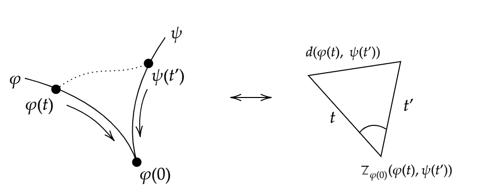
As our points approach the issue point, we will see this comparison angle approach some value.
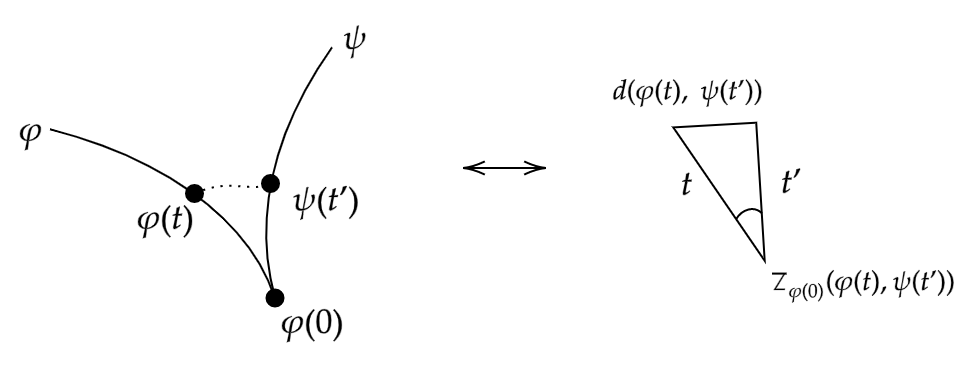
Of course this limit itself need not exist. One reason for this may be because the comparison angle may approach different values depending on whether \(t\) and \(t'\) approach \(0\) at different speeds. We will shortly see an example where this is the case.
Finally, note that this definition extends immediately to geodesic rays issuing from the same point. Essentially, the fact that our geodesic segments are of finite length plays no part in the above definition, as we only care about the behaviour of our geodesic as we approach the initial point. This idea is formalised by the germ of a geodesic (ray), but this formalism isn’t needed here.
We may wish to check that this definition of an angle falls in line with some of our basic intuition. For example, it should be clear that the angle between any geodesic and itself is \(0\). A similar question we might ask relates to the Euclidean idea that “straight angles” are \(\pi\) radians. We formalise this idea as follows.
Proposition 3.1. Let \(X\) be a metric space, and let \(\varphi : [a,b] \to X\) be a geodesic, such that \(a < 0 < b\). Define \(\rho_1 : [0,-a] \to X\) and \(\rho_2 : [0,b] \to X\) by
\[\rho_1(i) = -i, \ \rho_2(j) = j,\]then \(\angle (\rho_1, \rho_2) = \pi\).
The proof of this is relatively straightforward and a good exercise to get to grips with the definition. Another interesting property worth checking is that in Euclidean space, we can define a psuedo-metric (a metric that is not necessarily positive-definite) on the set of geodesics originating out of a point by measuring the angle between them. In particular, angles about a point in Euclidean space satisfy a triangle inequality. We will now show that Alexandrov angles also satisfy this same property.
Proposition 3.2. Let \(c\), \(c'\), and \(c''\) be geodesics issuing from the same point \(p\). Then
\[\angle(c', c'') \leq \angle(c', c) + \angle(c, c'').\]Proof. We will proceed by contradiction, and suppose that for some geodesics \(c\), \(c'\), and \(c''\) issuing from the same point \(p\in X\) such that \(\angle(c', c'') > \angle(c', c) + \angle(c, c'').\) Choose \(\delta > 0\) be such that
\[\angle(c', c'') > \angle(c', c) + \angle(c, c'') + 3\delta.\]By studying the \(\limsup\) in Definition 2.2, we can easily deduce that there must exist some \(\varepsilon > 0\) such that the following hold.
For all \(0 < t, t' < \varepsilon\), \(\overline \angle _p (c(t), c'(t')) < \angle (c,c') + \delta\),
For all \(0 < t, t'' < \varepsilon\), \(\overline \angle _p (c(t), c''(t'')) < \angle (c,c'') + \delta\),
There exists \(0 < t', t'' < \varepsilon\) such that \(\overline \angle _p (c'(t'), c''(t'')) > \angle (c',c'') - \delta\).
We now fix \(t'\) and \(t''\) such that (3) holds. Choose \(\alpha\) such that
\[\overline \angle _p (c'(t'), c''(t'')) > \alpha > \angle (c',c'') - \delta.\]Consider a triangle in \(\mathbb R^2\) with vertices \(x'\), \(x''\), and \(y\), such that \(\|x'-y\|_2 = t'\), \(\|x''-y\|_2 = t''\) and the interior angle between the segments \([y,x']\) and \([y,x'']\) is \(\alpha\).
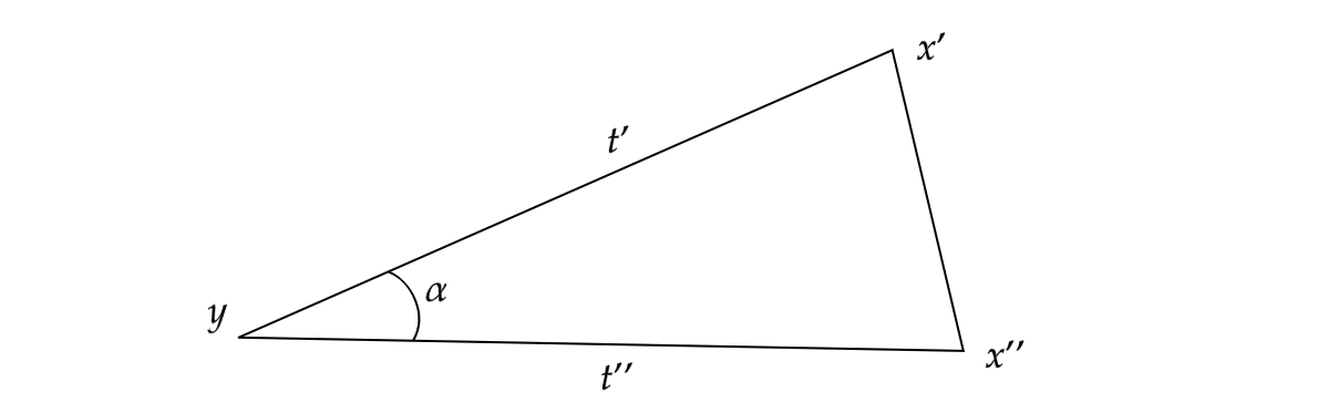
It is easily checked that \(\alpha \in (0,\pi)\), so we can safely assume that this triangle is non-degenerate (i.e. has non-zero area). From the definition of \(\alpha\), we can immediately infer that \(\|x'-x''\|_2 < d(c'(t'), c''(t''))\) by simply comparing our comparison triangle to the above. We can also infer \(\angle (c,c') + \angle (c,c'') + 2 \delta < \alpha\) from the lower bound of \(\alpha\). Using the latter of these two facts, choose \(x\) on the segment \([x',x'']\) such that the interior angle \(\alpha'\) between \([x,y]\) and \([x',y]\) is strictly greater than \(\angle(c,c') + \delta\), and similarly that the interior angle \(\alpha''\) between \([x,y]\) and \([x'',y]\) is strictly greater than \(\angle(c,c'') + \delta\).
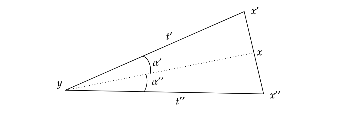
Let \(t = \|x-y\|_2\). By inspection we can deduce that \(t \leq \max\{t',t''\} < \varepsilon\). Thus we can apply (1) and deduce that
\[\overline \angle _p (c(t), c'(t')) < \angle (c,c') + \delta < \alpha'.\]By simply inspection this reveals that \(d(c(t),c'(t')) < \|x-x'\|_2\). Similarly, we may apply (2) and deduce that \(d(c(t),c''(t'')) < \|x-x''\|_2\). To finish, we may compute
\[\begin{align} d(c'(t'), c''(t'')) &> \|x'-x''\|_2 \\ &= \|x-x'\|_2 + \|x-x''\|_2 \\ &> d(c(t), c'(t')) + d(c(t), c''(t'')). \end{align}\]As this contradicts the triangle inequality in \(X\), our result follows. //
Remark. One might ask why we choose to take the \(\limsup\) over the \(\liminf\) for the cases where the angle doesn’t strictly exist. Part of the reason is that if we define our angles using the \(\liminf\), the previous proposition does not necessarily hold. I encourage the interested reader with some spare time to see if they can find an example where the proposition fails under the \(\liminf\) definition.
So we know that \(\angle\) defines a pseudo-metric on geodesics about some point \(x\). It is easy to see that this cannot be positive-definite, as one can imagine two distinct geodesics which are identical within some neighbourhood of $x$ and thus have an interior angle of \(0\). In fact there exist examples of pairs of geodesics, whose only common point is the shared initial point, which have an Alexandrov angle of \(0\).
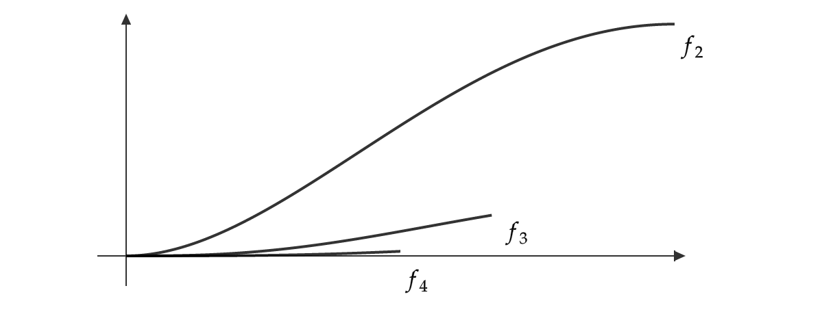
Example 3.3. Consider \(\mathbb R^2\) with the infinity-norm \(\| \cdot \|_\infty\). For every \(n \geq 2\), we define a geodesic \(f_n : [0,\frac 1 n] \to \mathbb R^2\) by \(f_n (x) = (x, [x(1-x)]^n).\) It is an easy exercise to check that each \(f_n\) is indeed a geodesic in \((\mathbb R^2, \| \cdot \|_\infty)\). Moreover, apart from the shared initial point these geodesics are pairwise disjoint. One can then use the fact that \(x \mapsto [x(1-x)]^n\) is a smooth function on \([0,1]\) with a \(0\) derivative at \(x = 0\) to argue that as these geodesics become arbitrarily “similar” as we approach the origin.
I leave the formal details to the reader but what follows is that we have an infinite number of pairwise disjoint geodesics issuing from origin, and the angle between any two is precisely \(0\).
We finish this section with a final example which demonstrates an example when these angles may not strictly exist.
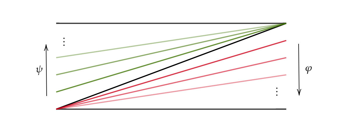
Example 3.4. Let \(X = C[0,1]\) be the space of continuous functions \([0,1] \to \mathbb R\), equipped with the supremum metric
\[\rho(f,g) := \sup _{x \in [0,1]} |f(x) - g(x)|.\]Consider the geodesics \(\varphi, \psi : [0,1] \to X\) defined by the formulae
\[\begin{align} \varphi(t)(x) &= (1-t)x \\ \psi(t)(x) &= (1-t)x + t. \end{align}\]These geodesics issue from the same point in \(X\), namely the identity function. \(\varphi\) is a path from the identity function to the constant function \(x \mapsto 0\), and Similarly \(\psi\) defines a path to the constant function \(x \mapsto 1\).
One can quickly check these are indeed geodesics in \(X\) by using the supremum metric to compute \(\rho(\varphi(t),\varphi(t'))\), and similarly for \(\psi\). If we fix \(t,t' \in (0,1]\), we can compute that
\[\rho(\varphi(t), \psi(t')) = \max \{t,t'\}.\]Thus, our comparison triangle at this point have side-lengths \(t\), \(t'\), and \(\max \{t,t'\}\). The comparison angle at \(\varphi(0)\) does not then approach any single value. Indeed, we can imagine that if \(t = t'\) then this comparison angle shall be \(\frac \pi 3\) as the triangle we have is equilateral. However, if for example \(t\) is much bigger than \(t'\), then this triangle becomes a “tall” isosceles, and our comparison angle approaches \(\frac \pi 2\). Thus, we arrive at an interesting situation where our Alexandrov angle does not strictly exist. Indeed all that matters here is the ratio between \(t\) and \(t'\). If we fix this ratio as we approach \(0\), we can make our comparison angle approach any value in \([\frac \pi 3, \frac \pi 2)\). Thus, in taking the \(\limsup\) we see that the true Alexnadrov angle between these two geodesics is \(\frac \pi 2\).
Recall that we say that a norm \(\| \cdot \|\) on a vector space \(X\) arises from an inner product if there exists some inner product \(\langle \cdot , \cdot \rangle\) such that \(\| v \| = \sqrt {\langle v , v \rangle}\) for all \(v \in X\). A norm which satisfies this condition can be seen as better behaved in terms of the geometry it induces. Indeed, an important result in linear algebra and functional analysis captures this by stating that a norm arises from an inner product if and only if that norm satisfies the parallelogram law. Formally, we have the following.
Proposition 4.1. Let \((X, \| \cdot \|)\) be a normed vector space. The norm \(\| \cdot \|\) arises from an inner product if and only if
\[\| v + u \|^2 + \| v - u \|^2 = 2\| v \|^2 + 2\| u \|^2\]for all \(v,u \in X\).
Alexandrov angles provide another alternative way to capture this idea of “well-behaved geometry”. As we will shortly prove, a normed space is an inner product space if and only if all Alexandrov angles about the origin strictly exist.
Before we can prove this result, we need to build up an understanding of geodesics within normed inner product spaces. First, we will show that normed vector spaces are geodesic, and that inner product spaces are uniquely geodesic.
Proposition 4.2. Every normed vector space is geodesic, and every inner product space is uniquely geodesic.
Proof. Let \(X\) be a normed space, and let \(v,u \in X\) be vectors. Let \(d := \| v- u\|\), and define \(\psi : [0,d] \to X\) by
\[\psi(t) = (1-\tfrac t d)v + \tfrac t d u.\]A quick calculation confirms that \(\psi\) is indeed a geodesic. Denote the above geodesic \([v,u]\).
We suppose that \(X\) is an inner product space so by the previous paragraph it is geodesic. Some thought reveals that showing \(X\) is uniquely geodesic is equivalent to showing that if \(x,y,z \in X\) satisfy
\[\|x-z\| = \|x-y\| + \|y-z\|,\]then \(y \in [x,z]\). It is then easily checked that this condition is implied by (and is in fact equivalent to) the condition that for all linearly independent \(v,u \in X\), we have that
\[\| u + v \| < \|u \| + \| v \|.\]We will show that inner product spaces satisfy this second condition. Let \(u,v \in X\) be linearly independent, so by the Cauchy-Schwartz inequality we have
\[|\langle u, v \rangle | < \|u\| \|v\|.\]We then compute
\[\begin{align} \| u + v \| &= \sqrt{\langle u+v, u+v \rangle} \\ &= \sqrt{\|v\|^2 +2 \langle u, v \rangle + \|u\|^2} \\ &< \sqrt{\|v\|^2 +2 \| u \| \| v \| + \|u\|^2} \\ &= \sqrt{(\| u \| + \| v \|)^2} \\ &= \| u \| + \| v \|. \end{align}\]It follows that all inner-product spaces are uniquely geodesic. //
With this fact in mind, we can now completely characterise inner product spaces using Alexandrov angles.
Theorem 4.3. Let \(X\) be a normed space, then \(X\) is an inner product space if and only if for all geodesics rays \(\varphi, \psi : [0,\infty) \to X\) issuing from \(0\), the Alexandrov angle \(\angle(\varphi, \psi)\) strictly exists.
Proof. We first show the ‘only if’ direction, so suppose that \(X\) is an inner product space and let \(\varphi, \psi\) be two geodesics as above. By Proposition 4.2, we know that \(\varphi, \psi\) are of the form
\[\varphi(t) = tu, \ \ \psi(t) = tv,\]for some unit vectors \(u\), \(v\).
Subspaces of \(X\) isometrically embed into \(X\), so let \(Y = \textrm{span}\{u, v\}\). Since Alexandrov angles are clearly a geometric property (invariant under isometry), we now need only show that \(\angle(\varphi, \psi)\) strictly exists in \(Y\). However, it is a well-known fact from linear algebra that all \(n\)-dimensional real vector spaces are isometric to \(\mathbb R^n\). Since that this angle clearly strictly exists in \(\mathbb R^2\), we are done.
Conversely, suppose that for all geodesics rays \(\varphi, \psi : [0,\infty) \to X\) issuing from \(0\), the Alexandrov angle \(\angle(\varphi, \psi)\) strictly exists. We will show that \(X\) satisfies the parallelogram law.
We choose two linearly independent unit vectors \(u,v \in X\), and consider the geodesic rays \(\varphi\), \(\psi\) defined by \(\varphi(t) = tu\), \(\psi(t) = tv\). Let \(\alpha = \angle (\varphi, \psi)\). We claim that for all \(t,t' > 0\), we have that
\[\alpha = \overline \angle_0 (\varphi(t), \psi(t')),\]i.e. that the comparison angle remains constant as \(t\) and \(t'\) approach \(0\). To see this, fix \(t, t' > 0\), then since the angle strictly exists we can say that
\[\alpha = \lim _{s \to 0} \overline \angle_0 (\varphi(st), \psi(st')).\]Applying the fact that \(\cos\) is a continuous function on \(\mathbb R\), as well as the law of cosines, we deduce
\[\begin{align} \alpha &= \lim _{s \to 0} \overline \angle_0 (\varphi(st), \psi(st')) \\ &= \lim _{s \to 0} \frac 1 {2s^2 t t'} (s^2t^2 + s^2 t'^2 - \| stu - st'v \|^2)\\ &= \lim _{s \to 0} \frac 1 {2t t'} (t^2 + t'^2 - \| tu - t'v \|^2)\\ &= \frac 1 {2t t'} (t^2 + t'^2 - \| tu - t'v \|^2)\\ &= \overline \angle_0 (\varphi(t), \psi(t')). \end{align}\]Thus our claim follows. We now have everything we need to show that the parallelogram law holds. We need only consider the linearly independent case, as the linearly dependent case is trivial. So let \(v\) and \(u\) be linearly independent vectors, and apply the previous claim to the unit vectors \(\frac v {\| v \|}\) and \(\frac {v+u} {\| v+u \|}.\) In doing so, we see that
\[\overline \angle_0 (v, v+u) = \overline \angle_0 (v, \tfrac 1 2 (v+u)).\]Applying the law of cosines to both sides of this equality, we get
\[\begin{align} &\frac 1 {2\|v\| \|v+u\|} (\|v\|^2 + \|v+u\|^2 - \|u\|^2 ) \\ &= \frac 1 {\|v\| \|v+u\|}(\|v\|^2 + \tfrac 1 4 \|v+u\|^2 - \tfrac 1 4 \|u-v\|^2 ). \end{align}\]From here it is a simple matter of rearrangement to show that the parallelogram law holds, and it follows that \(X\) is an inner product space. //
As an immediate corollary we may deduce that \(C[0,1]\) with the supremum norm is not an inner product space due to Example 3.4.
We will finish this section with a vague recollection of a faded memory - don’t inner product spaces have angles defined on them already? The answer is of course yes! Recall that the angle \(\alpha\) between two vectors \(u\) and \(v\) in an inner product space is usually defined by
\[\cos \alpha = \frac {|\langle u,v \rangle |} {\|u\| \|v\|}.\]If we associate a vector with its corresponding geodesic ray issuing from the origin, then it is not too difficult to check using the law of cosines that this definition of an angle between two vectors is in fact equivalent to the Alexandrov angle. I will however leave this as an exercise, as I found it relatively enlightening to see how the standard angle definition relates to the very geometric definition of Alexandrov angles.
If one is working with non-Euclidean spaces, such as hyperbolic or spherical spaces, there do exist standard “cosine laws” for these spaces which define angles in a more direct way. However, wonderfully it can be shown that these non-Euclidean cosine laws are in fact equivalent to the Alexandrov definition of an angle within their respective spaces. This post is already far too long, but a reader interested in exploring these ideas more should direct their attention to [1]. Specifically Proposition 2.9 of Chapter I.2 addresses this very question.
In fact much of this post has been adapted from parts of [1]. Thus if any reader craves a more official exposition of all discussed above, I would direct them to Chapter I.1 of the aforementioned text. This definition leads to the field of Alexandrov geometry, and the more-advanced reader who wishes to delve deeper into this area of mathematics is pointed towards [4] which provides a complete introduction to this field and its topics. Anybody looking to delve into the history of this generalisation may wish to track down the two seminal papers of this idea [2] and [3]. Do be warned however that these papers are not in English, and a brief history of the field is also presented in [4].
If anything discussed above is in need of clarification or correction, then I finally encourage the reader to point these issues out to me as soon as possible - either via the comments below or via email.
Bridson, M. R., & Haefliger, A. (2013). Metric spaces of non-positive curvature (Vol. 319). Springer Science & Business Media.
Alexandrov, A. D. (1951). A theorem on triangles in a metric space and some of its applications. Trudy Mat. Inst. Steklov., 38, 5-23.
Alexandrov, A. D. (1957). Uber eine Verallgemeinerung der Riemannscen Geometrie. Schriftenreiche der Institut fur Mathematik, 1, 33-84.
Alexander, S., Kapovitch, V., & Petrunin, A. (2019). An invitation to Alexandrov geometry: CAT (0) spaces. Springer International Publishing.
This post will be hopefully more accessible than other topics on this site, and should require no more than some basic set theory to comprehend. The contents of this post aren’t meant to be too thought provoking, as the point being made is quite moot. My aim is to demonstrate the (in my opinion) relatively nice combinatorial argument which falls out of this toy problem.
Edit, 26/7/2020: A small translation error has been corrected.
Hilbert’s Paradox of the Grand Hotel is a relatively famous mathematical thought experiment. It was introduced by David Hilbert in 1924 during a lecture entitled ‘About the Infinite’ [1, p. 730] (translated from the German ‘Über das Unendliche’). Hilbert’s goal in this demonstration was to show how when dealing with infinite sets, the idea that the “the part is smaller than the whole” no longer applies. In other words, the statements “the hotel is full” and “the hotel cannot accommodate any more guests” are not necessarily equivalent if we allow an infinite number of rooms. Hilbert gives the following explanation for how one can free up a room in an infinite hotel with no vacancies.
We now assume that the hotel should have an infinite number of numbered rooms 1, 2, 3, 4, 5 … in which one guest lives. As soon as a new guest arrives, the landlord only needs to arrange for each of the old guests to move into the room with the number higher by 1, and room 1 is free for the newcomer.
Indeed this can be adjusted to allow for any arbitrary number of new guests. For any natural number \(c\), we can accommodate an extra \(c\) by asking every current guest to move from their current room \(n\) to the room \(n+c\). Upon doing this, the rooms numbered 1 to \(c\) shall become available. Hilbert then goes on to demonstrate that we can extend this to even allowing an infinite number of new guests in our already full hotel.
Yes, even for an infinite number of new guests, it is possible to make room. For example, have each of the old guests who originally held the room with the number \(n\), now move into the one with the number \(2n\), whereupon the infinite number of rooms with odd numbers become available for the new guests.
This fact is somewhat remarkable and can seem rather counterintuitive upon first viewing. If we imagine ourselves standing in this hotel’s fictional foyer, the image of a corridor stretching off to infinity is sure to be a daunting one, and trying to make any kind of practical considerations within this setting is surely a fool’s errand. Alas that is exactly what the rest of this post shall try to do.
Suppose that we have our own grand hotel, and every room is currently occupied by a guest with a finite lifespan. We receive word that an infinitely long coach of tourists will be arriving shortly, and are asked to accommodate as many guests as possible. To accomplish this we may move guests between rooms as in the previous case, but with the catch that our current guests must arrive at their new room before their timely demise.
To explain further, consider the two examples laid out by Hilbert above. In the first case every guest simply moves one room along, possibly only a few meters (say \(x\) meters) away from their current room. This is an easy task that hopefully every guest will be able to accomplish within their lifespan. We have freed up 1 room with no dead residents. Success. Consider the second case however, where a guest in room \(n\) will have to move along \(n \times x\) meters to the room \(2n\). As \(n\) grows to infinity, this walk will of course become arbitrarily large and all but a finite number of our guests must perish en route to their new abode. Thus, while we have made an infinite number of rooms available, we have also caused the deaths of the majority of our guests. Not ideal.
Remark. Considering the second example, if we suppose that the rooms are 1 meter apart then the guest in room \(10^{27}\) will have to cross the observable universe in order to reach their new room.
Being the kind of mathematician to own an infinite hotel, we wish to optimise our potential income here. Thus we work will answer the question “how many rooms can we make available without killing any of our guests?”. One would hope that there is some clever system which would allow us to still free up an infinite number of rooms. However as we shall shortly prove, such a method does not exist. Requiring that our guests survive their journey between rooms is just much too grand a request if we wish to increase our hotel capacity by an infinite amount.
To formalise this problem, we will model it as follows. We will identify every room with its room number, and the hotel itself shall just be the set of room numbers. In particular our hotel is simply the set of natural numbers \(\mathbb N\). The movement of current guests shall be modelled by a function \(f : \mathbb N \to \mathbb N\). Of course every guest must be assigned a unique room, and so we add the requirement that \(f\) is injective. If we let
\[E_f := \mathbb N \setminus \text{Im} f\]denote the set of rooms left available after applying \(f\), we can see that our goal is to maximise the order of \(E_f\).
In adding the requirement that guests cannot walk “too far”, we are stipulating that for all \(n \in \mathbb N\), \(|f(n) - n |\) cannot grow too large. To simplify things slightly, we will assume every guest has one universal maximum walking distance, say \(c\). Thus we wish to bound
\[|f(n) - n | \leq c\]for every \(n \in \mathbb N\). We will say that a function satisfying this condition is relatively bounded by \(c\).
Remark. Note that the term ‘relatively bounded’ as it is used here is by no means standard, and is simply being defined here for convenience.
Returning to Hilbert’s examples once again, if we consider the first case where we move every guest to the next room over we can see that \(|E_f| = 1,\) and that \(|f(n) - n | = 1\) for all \(n\). In the second case, we have that \(E_f\) is countably infinite, but for every \(n\) we have that \(|f(n) - n | = n,\) which grows arbitrarily large. This breaks our imposed condition that \(f\) be relatively bounded, and so this strategy is not valid.
Clearly we can accommodate \(c\) new guests by mapping \(f(n) = n+c\) as discussed earlier. Our claim is that this is the best one can do under these mortal circumstances.
We shall model our choice of \(f\) as follows. Suppose we have a warden who walks down the corridor, knocking on each door in turn and telling the residents to which suitable room they must move. This warden has a list of all rooms, which are initially all marked as “FREE”. Upon telling somebody to move to room \(m\) the warden shall mark it as “OCCUPIED” on their list, and this room will no longer be considered for later moves. The warden also begins with an empty list of “EMPTY” rooms. If the warden is currently relocating resident \(n\) with the room \(n - c\) marked as “FREE”, and the warden does not choose this room, then they shall add \(n - c\) to their “EMPTY” list before moving on. The intuition behind this is that if room \(n - c\) is not chosen for resident \(n\) or earlier, then it will never be chosen and shall remain empty until the new guests arrive.
With this combinatorial model of \(f\), it is clear that our goal is to grow the “EMPTY” list. However, note that this list only grows in a very specific circumstance. This observation will allow us to prove our claim.
Theorem 1. The order of \(E_f\) for any injective function \(f : \mathbb N \to \mathbb N\) which is relatively bounded by \(c\) is no larger than \(c\).
Proof. We will apply our ‘warden’ model, and proceed by induction to show a slightly stronger claim. We will show for all \(n \in \mathbb N\) that if the warden has \(l\) rooms on their “EMPTY” list, and is knocking on the door of room \(n\) with \(k\) suitable “FREE” rooms which this resident can be relocated into, then
\[l + k = c+1.\]Since \(k\) is always at least 1 (room \(n+c\) is always free), our claim follows. To simplify the induction without loss of generality, we suppose that the hotel is padded with \(c\) ‘dummy’ rooms to the left of room 1, which are permanently occupied. This removes the need to treat the first few cases as somehow different because they aren’t surrounded by \(2c\) other rooms.
For the base case, suppose that the warden is knocking on the door of room 1. Currently their “EMPTY” list contains 0 rooms, and the number of rooms to which this resident can be moved to is \(c+1\). Our claim thus follows trivially.
Next, we shall perform the inductive step. Suppose the warden has \(l\) rooms on their “EMPTY” list and is knocking on the door of room \(n\) with \(k\) suitable “FREE” rooms which this resident can be relocated into, such that \(l + k = c+1\). We have two cases.
Case 1. Suppose room \(n-c\) is not currently free. Inspection reveals that every room which is “FREE” near room \(n\) is also then near room \(n+1\). However, resident \(n\) must then be allocated a room from the pool of rooms which resident \(n+1\) is choosing from next. Since resident \(n+1\) can also choose room \(n+c\) (which is guaranteed to be free), they shall be choosing from \(k - 1 + 1 = k\) rooms. The “EMPTY” list remains of length \(l\), and it follows that our claim also holds when the warden knocks on door \(n+1\).
Case 2. Suppose instead that room \(n-c\) is currently free. In this case, one can see that every “OCCUPIED” room which was in range of room \(n\) must also have been in range of room \(n+1\). We now consider two subcases.
First suppose the warden chooses \(f(n) = n-c\). Then the new room that resident \(n\) occupies will not be within range of room \(n+1\), and so it follows that resident \(n+1\) will also have \(k\) possible rooms to choose from. Since the “EMPTY” list remains at length \(l\), our claim follows.
If instead \(f(n) \neq n-c\), then this means \(n-c\) will be added to the “EMPTY” list, and the list will now be of length \(l' := l+1\). In this case, resident \(n\) shall now occupy a new room within range of \(n+1\). This will reduce the number of possible choices for \(f(n+1)\) by 1. Thus when the warden knocks on the next door, there will only be \(k' := k - 1\) suitable free rooms to choose from. We finally have that
\[k' + l' = k + l -1 + 1 = k + l = c+1\]as required.
It follows that this list of “EMPTY” rooms can only contain at most \(c\) rooms, and our theorem is proven. //
Edit, 27/7/2020: Better arguments for the above have since been demonstrated. I’d encourage the reader to try figure out a shorter proof for themselves, otherwise some of these arguments can be found in this reddit thread.
As it turns out, if we add the restriction to Hilbert’s thought experiment that our guests are all mere mortals, then a full hotel can only accommodate a finite number \(c\) of new guests. With a goal of estimating this value \(c\), I will finish this short article with some napkin mathematics. Combining some assumptions about the guests staying at our hotel with some hastily googled statistics, I will try to pull out some concrete numbers about our hotel’s optimal performance. After all, we know that \(c\) is finite, why not try calculate it?
Suppose that we have full control over who we let stay in our hotel, in that every room contains a human perfectly optimised for relocation to the furthest room possible. I will take this as a female toddler with an age 18 months old, since females tend to live longer and most children can walk fairly confidently by this age. Countries exist with a female life expectancy of ~90 years (Monaco, for example), so we shall assume that our guests all share this lifespan of 90 years. This means we can expect the Monégasque toddlers in our hotel to live for a further 88.67 years, or 2,796,300,000 seconds.
The average walking speed of a human being is 1.4 meters per second. Let us assume that the distance between rooms is about 3 meters (this is not a luxury hotel). Calculation then tells us that it would take a person on average 2.14 seconds to travel from one room to the room next door. Putting these numbers together, we see that during the rest of their lifespan, our guests can walk up to 1,306,682,243 rooms away. By Theorem 1, it thus follows that this hotel could only accommodate 1,306,682,243 new guests before existing guests began to die on their journeys.
I believe this provides a relatively sound upper bound to how many new guests Hilbert could actually accommodate. Indeed 1,306,682,243 is less than infinity, and in fact is actually less than the population of India. If anybody dreaming of becoming a transfinite architect is reading this, don’t let this reality check demotivate you. Follow your dreams.
I don’t intend for this to be a definitive guide to the application process, as I could never claim that my application was perfect. However, I do know that when I was applying I found it difficult to find people openly discussing their own experiences with the application process (especially for this programme which features a relatively small cohort of ~17 people per year). Thus, if just one person in future years finds this post useful when writing their own application, then this summary was worth writing.
If you are reading this, then I will presume that you would like to apply for the MFoCS at Oxford (or another related programme) and are seeking advice. I will briefly summarise the programme for the less-informed reader, to give context to the rest of this post.
The Oxford MFoCS is the University’s MSc in Mathematics and Foundations of Computer Science. It is a taught programme which runs for 12 months, beginning in Michaelmas term and running into the Summer. The programme is assessed by 5+ mini-projects (extended essays) and a dissertation in the Summer term. Regarding the contents of the course, I will quote the University directly.
The [MFoCS], run jointly by the Mathematical Institute and the Department of Computer Science, focuses on the interface between pure mathematics and theoretical computer science. The mathematical side concentrates on areas where computers are used, or which are relevant to computer science, namely algebra, general topology, number theory, combinatorics and logic. Examples from the computing side include computational complexity, concurrency, and quantum computing.
This programme is a natural fit to anybody coming from a mathematics degree, with any level of interest in the mathematics behind computer science. In this post, I will summarise some key points from my academic CV, statement of purpose, and finally the interview. I will also talk a bit on what followed, hopefully giving some clues to how long the admissions process may take.
Though a very important part of the application process, I will not discuss referees here. An application requires three referees, with at least two being academic in nature (all three of mine were academic). Your referees should be people who can speak confidently about your ability. Other than that, your choice of referees will vary greatly depending on your own prior experience/networking, and there is nothing I can say here to really advise on this.
This was probably the first thing I finished working on during my application. I do not believe that too much weight is placed on the CV, and so I would suggest not spending too much time on this. The official guidance states the following.
A CV/résumé is compulsory for all applications. Most applicants choose to submit a document of one to two pages highlighting their academic achievements and any relevant professional experience.
That being said, my CV was split into five sections across two pages, namely Education, Relevant Employment, Writings, Technical Skills, and Other Awards. These headings are mostly self-explanatory, and the key point to take away is to keep things relevant. Any education will of course be relevant, but employment should be restricted to research, teaching, and anything else which the department might view as appropriate (something related to mathematics and/or computer science would fit this mould).
Regarding the Writings section, this might usually be called Publications, but as an undergrad you will not be expected to necessarily have many, if any, peer-reviewed pieces to your name. I personally had no publications I could mention at the time of applying, so this section for me included this blog, and a project report from a recent research internship which was due to be edited into a publication later that year. I made this report available online for the department to read should they so wish – indeed if it cannot be accessed, it might as well not be on there.
Finally, Technical Skills and Other Awards should again be self-explanatory titles, and the relevancy rule still holds. For my application, the relevant skills I could present were my programming ability, and a proficiency with LaTeX. The latter section might then contain any academic awards one has earned, however big or small.
The Statement of Purpose (SOP), also known as the Personal Statement, will take up the bulk of your time in applying. I will again quote the admissions page for context on what they are looking for.
Your statement should be written in English and explain your motivation for applying for the course at Oxford, your relevant experience and education, and the specific areas that interest you and/or you intend to specialise in. This will be assessed for your reasons for applying; evidence of motivation for and understanding of the proposed area of study; the ability to present a reasoned case in English; and commitment to the subject, beyond the requirements of the degree course. Your statement should focus on your motivation for wishing to undertake the course rather than personal achievements, interests and aspirations.
My SOP was written using Overleaf, fitting within one page of A4 paper with a 1” margin and 11pt font. Of course any other word processor will do just as good a job however (just make sure it’s exported as a PDF file). I personally split my SOP into 6 paragraphs, each of which I will now summarise independently.
An introduction/summary, within which I briefly stated where I was coming from, where I wanted to be, and how the programme I was applying for would help to bridge that gap. You will be assessed on your reasons for applying so it is good to make your motivations clear from the first couple of sentences.
To demonstrate my own “commitment to the subject beyond the requirements of the degree course”, my next paragraph summarised my own (relevant) extra-curricular readings and writings. This included a summary of this blog and its goals, as well as a selection of appropriate texts I had read. It is incredibly important that anything you claim to have read, you must have actually read (or can at least talk confidently on its contents), for reasons which will be discussed in the next section. I also suggest you not just say what you have read, but briefly justify why with what you hoped to get out of it. I also mentioned some reading groups that I was part of which focused on topics pertinent to the programme I was applying for, mainly in the computer science department. I will also remind the reader that the assessors do not want to see a reading list, your goal should be to demonstrate your commitment with technical knowledge beyond that required by your curriculum.
The third paragraph followed with a similar tone, where I aimed to summarise my own relevant work experience. For me, this took form of teaching and research, and I would be careful when mentioning anything but these categories (as mentioned earlier). The goal here is again to demonstrate commitment to the subject, and I would recommend that anything one writes in this section, they somehow tie back to their case for why they should be considered. In this paragraph I also give a relatively technical summary of the aforementioned research, expecting to be asked about it at interview. Your assessors will be mathematical academics themselves, so do not shy away from discussing specifics.
I included a short paragraph detailing my final-year project. Outside of your references, this may be your only chance to tell the assessors about your project. Again, I chose to give some level of technical detail in this brief exposition, expecting to discuss it further at interview.
This paragraph may have been one of the most important. Here I summarised my own intended pathway through the MFoCS. I did this by detailing units I was interested in taking, including stating why I was interested and also pointing out how I would meet the prerequisite knowledge for my choices. I believe that the assessors really want to see that you have done your research regarding the programme, and know exactly what you are applying for. This is where I took the opportunity to state “the specific areas that interest [me] and/or [I] intend to specialise in”, in their words.
I chose to conclude my SOP with a short, sharp summary. I’m not sure how important this really is in the bigger picture, but I figured a couple sentences bringing together the key points I had made towards my case in the earlier paragraphs could only help deliver a “reasoned case”.
This layout is of course not the only, nor the best layout possible. I suggest you actively move your paragraphs around until you find a nice flow in your own argument, as that is what you are essentially writing – an argument.
My application was marked as ‘ready for assessment’ on January 7th 2020 and I received an invitation to interview on March 6th, totalling to just under 8 weeks of waiting. I chose to attend my interview in person, which took place at the Department of Computer Science the following week on March 11th. I had two interviewers, and was told their names in advance.
Regarding preparation, I chose to spend my time reading about my interviewers and their own research interests, as well as making sure I knew my own application materials by heart. I made sure I could speak confidently about any literature I had mentioned in my SOP, and made sure I could recall some technical definitions in the works I was less familiar with.
The interview lasted exactly 30 minutes, and was more of a discussion about my application than I anticipated. While many questions asked were technical in nature, I was not asked any particular “test” questions like you might get in a typical undergraduate interview. Your mileage may of course vary, and they do say to expect an interview which is “mainly technical questions”. The interview took the format of walking through my SOP step-by-step, being asked to elaborate on each bit. For example, I was asked about a reading group I had mentioned, and was asked to give a result which we had recently encountered in these sessions. I was also asked to give specific details about some parts of my project which had been mentioned in the SOP.
Sidenote: A personal highlight from my own interview was being asked whether a particular result being discussed was recently discovered or more classical, and I was able to name both the finder and its year of publication.
What I believe to be common in every interview is that I was quizzed on what I knew about the programme. In particular, its structure and I was asked to give some units which I might be interested in taking, which were then discussed. One of the units I chose to mention was actually currently being lectured by one of my interviewers, and I chose to point this out in order to demonstrate that I had genuinely read into the specifics of these units.
A piece of advice I was told before the interview was to know my own research back-to-front and to be able to talk about it fluently. This turned out to be incredibly wise advice, as one of my interviewers was familiar with the area I had worked in. I was asked to formally state a result which I had found, and to try give some intuition to its statement. A second piece of advice I was given was to never try to lie about anything anywhere near your interviewers’ research areas. For example, claiming to have read a paper of theirs will get you quizzed on that paper, and you will be found out if you haven’t done your homework (however, if you have done your homework this can be a great technique to get things moving).
At the end of the interview you are typically given a chance to ask your own questions. I had two questions prepared, one for each of the interviewers. One of these was a technical question relating to a recent paper which I had read by one of them, which was received relatively well and opened up a brief discussion. The other was a question about a textbook written by the second interviewer, of which I had read the first chapter before the interview. Again this was relatively well received, and led to into a discussion about one of the units on offer.
This summary may or may not be representative of the general interview experience, and I suspect it depends hugely on who your interviewers are. However, I also suspect that they choose your interviewers based on whose research interests align with your own. Thus, you should hopefully not struggle to find common ground to start up a conversation (provided you have done your research).
Following the interview, there was radio silence until March 20th, just over a week later, when I received my offer by email. You are then asked reply to your offer and subsequently complete a criminal convictions declaration.
In the next few months, you will be allocated a college. If you indicated a preference of college in your application, then this college will consider your application first but may or may not decide to take you. If they decide not to, you will usually find out relatively quickly and will be placed into a pool of other postgrad students waiting to be allocated a college. If you did not indicate a preference, you will simply be placed straight into this pool.
The wait times then vary massively. I know many people who received a college offer very shortly after applying. I also know people (including myself) who were left waiting for 12+ weeks after their departmental offer to find out their college. I would advise patience in this wait, but given accommodation arrangements often depends massively on college, this period can be relatively stressful.
I received a college offer on June 15th from Balliol College, just over 12 weeks after my departmental offer. I did not indicate a preference on my application.
Upon receiving a college offer, you will be asked to submit a financial declaration. This is a form simply asking for evidence that you are able to pay for your course fees. Beyond this, your timeline will depend entirely on the college you are allocated and so my summary shall stop here.
Overall, my advice falls into two categories. Keep your application relevant, and make sure you are something of an expert on every part of it (including your interviewers). The interview will probably be more chill than you are expecting, but that doesn’t mean you shouldn’t prepare to the best of your ability. Finally, as always you should understand that these programmes are often ludicrously competitive, and rejection does not bear negatively on yourself. The official graduate admissions statistics for the Mathematical Institute can be found in this FOI request, and they do a good job at demonstrating just how competitive this department can be.
If you have any further questions regarding anything above, then feel free to either leave a comment or drop me an email.
]]>This budget allows you to input your expected incomes and expenditures for the year ahead, and forecast your balances through the next 12 months. This sheet is especially suited to students, allowing you to know in advance if you’re heading towards your overdraft (or beyond) later in the year.
The template can be found here. This link will lead to a prompt to copy the file, following which the sheet will most likely be available within your ‘My Drive’ folder. The rest of this post will be a brief summary of the functionality available. One will note that there is two different templates – one with investments and one without. These are mostly identical but with some small additions in the former to allow the user to track an investment portfolio as well. This guide will focus on the latter, with an addendum on the former.
First things first, only cells with red font should be editted by the user, and any others left to be automatically filled in. This sheet tracks two balances for the user - a main spending account and a savings account. All spending and income is assumed to be coming in and out of the main account, with the savings account remaining untouched apart from the occasional deposit or withdrawel. The sheet is split vertically into four sections. They are PLANNED, RECORDED, PROJECTED, and MISC.
Each column of the sheet represents a week, with the date at the top being the first day of that week. Choose your start date in the bottom-left corner under MISC. and the rest of the year will be filled in. The current week will be highlighted in yellow for visibility. We will now take a more in-depth look at the first three of these sections.
The PLANNED section is where you should input all of your expected incomes and expenditures throughout the year, separated by category. For example, if the user has a student loan coming in on 21/4/2021 of £2000, they should find the week containing 21/4 and enter 2000 in the Student loan row. If Spotify will be charging the user £5 on 11/1/2021, they should enter -5 in the Subscriptions row under the relevent week. One should fill this section in to the best of their knowledge at the start of the budget to make projections/forecasts as accurate as possible, but of course one can edit this section through the year too as their financial situation changes. Note that the Living costs section will be already filled in, containing a default weekly budget which the user can set under the MISC. header. This can of course be overridden if a particular week is expected to be particularly cheap or expensive. Note that rows can be renamed, added, and removed from this section easily to suit the users own needs.
The RECORDED section is where one should record their balances at the end of every week. As mentioned earlier, this sheet is set up to contain two balances – a main spending account and a savings account. The user should input the total balances of these accounts after each week, which will then subsequently be compared to the forecasted balances to see whether you have overspent or underspent that week. For example, if you have reached the end of the week commencing 3/2/2021 with £2030 in your main spending account and £405 in your savings, you should enter these values under 3/2 in the RECORDED section.
Finally the PROJECTED section does not require much input at all. Here data from previous weeks is combined with expected spending taken from PLANNED to predict future balances. There is one row which allows inputs, that being the Exp. savings deposit which allows you to tell the sheet if you are planning to move your own money around in the future. For example, if you know that in the week of 6/12/2020 that you’ll need to take £200 out of your savings to help pay for Christmas, you can enter -200 in this section. Similarly, if you plan to move £500 into your savings in a particular week, you can enter in this row to make sure that is taken account of in any projections.
If the user wishes, the sheet can also track their investment portfolio. In principle, this functions the same as having a second savings account being tracked separately, but with a small difference. One can set an expected weekly gain under the MISC. heading. This value is defaulted at 1%, meaning you expect your portfolio to increase in value by 1% every week.
One also has a new Exp. investments section which functions identically to the Exp. savings deposit and allows the user to input whether they expect to move money from their main account into their investments or vice versa.
There is then nothing else that the user needs to input themselves, and from here the sheet will plot a graph projecting your balances through the rest of the year. Under MISC. the Future main acc. low value simply records how low your main account is projected to hit in the future, and serves as a good indicator as to whether you are able to move some money into savings, or on the other end of the spectrum are heading towards your overdraft (or are simply running out of money). The second graph will fill out through the year, and tracks how over/under budget your spending has been so far.
Everything else within this sheet is hopefully self-explanatory, but if you have any questions about it then feel free to drop me an email or a comment below.
]]>For the sake of brevity, I will assume a working knowledge of combinatorial group theory and group presentations, however an informal exposition will be provided in Section 1.
Very briefly we shall restate some important definitions and results regarding group presentations with the goal of building up to our main question, the reader who is familiar with such notions can safely skip this section. We will be roughly following the definitions laid out by Magnus in [1]. Combinatorial Group Theory is the study of defining groups with a set of generators, and another set of words in these generators known as relators. More formally, we have the following definitions.
Definition 1.1. (Words) Let X be a set of n symbols and for any symbol \(x\) in X, define its formal inverse as a new symbol \(x^{-1}\). Similarly, the inverse of a symbol \(x^{-1}\) is defined as just \((x^{-1})^{-1} = x\). Let X* be the set of words in these symbols and their inverses (including the empty word, denoted 1), where a word is a finite sequence of symbols. Furthermore, define the formal inverse of a word w in X* as
\[w^{-1} = (x_1 x_2 \ldots x_n)^{-1} = x_n^{-1} \ldots x_2^{-1} x_1^{-1}\]where each \(x_i\) is either an element of X or the inverse of one. Given two words w and v, we define their juxtaposition wv as concatenation in the obvious sense. A word v is a subword of another word w if it itself appears as a contiguous block within w. We may parameterise a word \(w(x,y,z \ldots)\) or \(w(X)\) to denote the set of symbols appearing in w.
Definition 1.2. (Group presentations) Let X be a set of symbols, then a presentation is a pair \(\langle X ; R \rangle\) where R is some subset of X*. Elements of X are known as generators, and elements of R are known as relators.
We say two words w and v in X* are equivalent if v can be obtained from w by a finite sequence of the following operations.
Insertion of any element of R or its inverse, or a string of the form \(xx^{-1}\) or \(x^{-1}x\) where \(x \in X\), in between any two consecutive symbols, or at the beginning or end of the w.
Deletion of any element of R or its inverse, or a string of the form \(xx^{-1}\) or \(x^{-1}x\) where \(x \in X\), if it appears as a subword of w.
This forms an equivalence relation on X* (we will not check this here), and it is clear that any relator lies within the class of the empty word. Define the following operation on the set of equivalence classes,
\[[w] \cdot [v] = [wv],\]where v, w are elements of X*, and indeed this forms a group with the class of the empty word as the identity, and the obvious inverses (which is another fact we will not check). Given some presentation P, denote its equivalence class group \(\overline{P}\). One can think of relators as equations, where if the word R is a relator, then we stipulate \(R = 1\) within our group. We may sometimes abuse notation and write relations \(X = Y\) instead of relators in our group presentations, but it isn’t hard to see that this doesn’t change anything (every relation can be re-expressed as a relator). If a relation holds in a group given by a presentation, then this relation is said to be derivable from the given relations.
We have that every presentation defines a group, and in fact it is also true that every group is defined by some presentation. More precisely we have the following theorem.
Theorem 1.1. (Equivalence of groups and presentations) Let G be some group, then there exists a presentation P such that G is isomorphic to \(\overline{P}\). Furthermore, every presentation defines a group in the above way.
So our notions of presentations and groups are indeed equivalent, though a given group may have many different presentations. A group G is called finitely generated if there exists a presentation for G with a finite set of generators, and similarly a group is called finitely presentable if there exist a presentation for G with both a finite set of generators and relators. The goal of this post is to work towards an example of a group which is finitely generated but not finitely presentable, and demonstrate that these two conditions are indeed very different.
We shall consider a result presented by B. H. Neumann, in his 1937 paper Some remarks on infinite groups [2]. This result about finitely presentable groups will be used in Section 3 to argue that our construction cannot be finitely presentable, by contradiction.
Theorem 2.1. Let G be a group defined by the finite presentation \(\langle x_1 \ldots x_n ; R_1, \ldots R_m \rangle\), and some suppose that \(Y = \{y_1, \ldots y_l\}\) is another finite generating set of G. Then, G can be defined with finitely many relators in Y.
Proof. Write \(X=\{ x_1 \ldots x_n \}\), we consider the following sequence of transformations. First, we write each \(x_i\) in terms of Y, and vice versa, as both X and Y generate G. That is,
\[x_i = X_i(Y), \ \ y_j = Y_j(X),\]for some words \(X_i\), \(Y_j\), for all i, j. Now we can transform G’s finite presentation in X by adding each \(y_j\) as a generator, and adding the relation \(y_j = Y_j(X)\), for each j. We then add the relations \(x_i = X_i(Y)\) to our presentation, for each i (these should not change the group as they are derivable from existing relations). Using these new relations, we then substitute \(X_i(Y)\) for each appearance of \(x_i\) in the old relations. Following this, each \(x_i\) is defined in terms of Y, and do not form part of any other relation in the presentation. It follows that we can delete generators X from our presentation as well as the corresponding relations, leaving us with a finite presentation of G in terms of generators Y. //
Remark. It is not too hard to see how the above result can be improved to a bound on the number of relations required to define G, and this is in fact what Neumann does in his paper.
Corollary 2.2. Suppose G is finitely presentable, and let \(\langle y_1, \ldots y_n ; S_1, S_2, \ldots \rangle\) be a presentation for G with finitely many generators, but infinitely many relators. Then, there exists an l such that \(\langle y_1, \ldots y_n ; S_1, S_2, \ldots S_l \rangle\) also defines G. That is, all but finitely many of the relators are redundant.
Proof. Write \(S = \{S_i \ ; \ i \in I\}\), and recall that since S is a defining set of relators, every other relator in G is derivable from S. In particular, every relator in G can be derived in a finite number of applications of the rules (1) and (2) mentioned in Section 1. Let \(\langle Y ; R \rangle\) be some finite presentation of G in generators Y, which must exist by Theorem 2.1, then every relator in R is derivable from S in a finite number of steps. Since R is itself finite, we must have that every relator in R can be derived using only a finite number of relators in S. Then, since every relator of G can then be derived from R, it follows that every relator of G can be derived using just a finite subset of S, and thus all but finitely many relators in S are redundant. //
We will now see how the above corollary can be used to show that a particular group defined by just two generators cannot be finitely presented. This example is a simplified version of Neumann’s example, and is borrowed from [3]. We need to take a look at a concrete example of a group, the alternating group, but before that, a quick lemma on conjugate cycles.
Lemma 3.1. Let \(\rho = (a_1, a_2, \ldots a_s)\) be a cycle and \(\pi\) be a permutation in \(S_n\). Then
\[\pi \rho \pi^{-1} = (\pi (a_1), \pi (a_2), \ldots \pi (a_s)).\]Proof. Let b be any symbol, and first suppose b does not equal \(a_i\), for any \(i\). Then we have \(\pi \rho \pi^{-1} (b) = b,\) and we are done. Else, fix some \(i \leq s\) and observe that \(\pi \rho \pi^{-1} (\pi(a_i)) = \pi \rho (a_i),\) so in the cycle decomposition of \(\pi \rho \pi^{-1}\) we have that \(\pi(a_i)\) sits to the left of \(\pi(\rho(a_i))\). Recall that in \(\rho\), \(a_i\) sits to the left of \(\rho(a_i)\), so in fact since \(i\) was chosen arbitrarily we have
\[\pi \rho \pi^{-1} = (\pi (a_1), \pi (a_2), \ldots \pi (a_s)),\]as required. //
We now turn our attention to the commutativity of certain elements of the alternating group. The proof of the next lemma is adapted from this answer on Mathematics Stack Exchange.
Lemma 3.2. Let \(j \geq 7\) be an odd integer, and let
\[\alpha = (1, \cdots j), \ \ \beta = (1, 2, 3)\]be cycles in the alternating group \(A_j\). Then \(\alpha^k \beta \alpha^{-k}\) commutes with \(\beta\) if \(3 \leq k \leq j-3\), but not if \(k = j-2\).
Proof. From Lemma 3.1, we can deduce that
\[\begin{align} \alpha^k\beta\alpha^{-k} &=\left(\alpha^k\left(1\right),\ \alpha^k\left(2\right),\ \alpha^k\left(3\right)\right)\\ &=\cases{\left(k+1,\ k+2, \ k+3\right)&if $\ 1\le k\le j-3$,\\ \left(1,\ j-1, j\right)&if $\ k= j-2$.} \end{align}\]The remaining cases are not important. It is clear from here that if \(3 \leq k \leq j-3\), we have that \(\beta\) is completely disjoint from \(\alpha^k \beta \alpha^{-k}\), and therefore these two elements must commute. As for the case where \(k = j-2\), we calculate that
\[\beta \alpha^k \beta \alpha^{-k} = (1,2,3) (1, j-1, j) = (1,2,3,j-1,j),\]whereas
\[\alpha^k \beta \alpha^{-k} \beta = (1,j-1,j) (1, 2,3) = (1,j-1,j,2,3).\]Our result follows. //
From here, we can prove our main result. A final notational remark, we notate the commutator \([x,y] := xyx^{-1}y^{-1}\). Recall that \([x,y] = 1\) if and only if \(x\) and \(y\) commute.
Theorem 3.3. There exists a finitely generated group which is not finitely presentable.
Proof. Consider the group G defined by the presentation
\[\langle a, b ; [a^{2k+1} b a^{-(2k+1)}, b], k \in \mathbb N \rangle,\]and suppose G is finitely presentable. To ease notation, write \(c_k = [a^{2k+1} b a^{-(2k+1)}, b]\), and consider the group \(A_{2l+3}\), for \(l \geq 2\). If we then consider the map \(a \mapsto \alpha\), \(b \mapsto \beta\), then it follows from Lemma 3.2 that for \(1 \leq k \leq l-1\), \(c_k = 1\) in \(A_{2l+3}\), but \(c_l\) does not equal 1. It follows that the relation \(c_l=1\) can’t be derived from \(c_1, \ldots c_{l-1}=1\) (if it could then \(c_l\) must equal 1 in \(A_{2l+3}\)). Since this is true for arbitrary \(l \geq 2\), this contradicts Corollary 2.2, and so G cannot be finitely presentable. //
In [2], Neumann uses this result (with his slightly fancier example) to go on to show that there are in fact uncountably many groups defined with two generators, up to isomorphism. Of course, there are only countably many finitely presented groups up to isomorphism, so in fact even for finitely generated groups, being is finitely presentable is far from the norm.
I have written this up, slightly adapting [3], as a small aside while I work on my project this year. My project concerns decision problems within combinatorial group theory, and indeed [3] (as well as much more literature) has formed a good part of my current reading.
Magnus, W., Karrass, A. and Solitar, D., 1976. Combinatorial Group Theory. Dover Publications.
Neumann, B.H., 1937. Some remarks on infinite groups. Journal of the London Mathematical Society, 1(2), pp.120-127.
Button, J., and Chiodo, M., 2016. Infinite groups and decision problems. Lecture notes, University of Cambridge. Link.
I have written this piece with the goal of not requiring any prior knowledge of quantum computation - but will be assuming a good working knowledge of linear algebra and complex vector spaces. I also assume knowledge of Big-O notation though this is fairly self-explanatory in context.
Consider the problem of finding a particular marked item in an completely unsorted list. With no structure or order to abuse, the only option we are left with is essentially checking each element of the list one-by-one, hoping we come across our marked entry at some point in the near future. It’s easy to argue that in a list of N items, we would need to check an expected number of N/2 items before we come across our item, and N-1 to find it every time with certainty.
Of course in a sorted list, we could do much better using techniques like binary-search to improve our number of queries to O(log N). Sadly this is of no use to us here, and if we wish to gain any kind of speed-up to this process we will need to leave the realms of classical computation.
In 1996, Lov Grover presented his revolutionary quantum search algorithm [1], which makes use of quantum mechanics to find the marked item with high probability, using only \(O(\sqrt N)\) queries. This is quite the result. For some concreteness consider an unsorted list of 1,000,000 elements. Classically, to find our marked item we would have to check pretty much every element in the list, in the worst case. However, Grover’s algorithm would find the marked item with roughly 800 queries to this list - a very dramatic improvement. There is some subtlety as to what we mean by a query in the quantum case, but we will discuss this in section 3.
In this section we will provide a brief description of quantum computation in general, for some context to the algorithm. First, lets consider classical, deterministic computation. We will have a system that starts in some initial state - say a binary register set to 00…0 - and our algorithm will change this state to another state. The system will only ever be in one state at any given moment but may cycle through plenty of different states over time while the algorithm computes. Every choice the algorithm makes is completely deterministic, and so our algorithm is essentially a function mapping from states to states. However, it need not be this way.
Grover [1] describes quantum computation with an analogy to probabilistic algorithms. Consider an algorithm that flips a coin at some point(s), and decides what to do next based on the result(s). We can then model the outcome of the algorithm (as well as all intermediate steps) with a probability distribution of possible states that the system could be in. In particular, the state of the system could be described by a vector \((p_1,\ldots,p_N)\) where each component contains the probability of being in a particular state at that point in time (note that we can think of the standard basis vectors \((1,0,\ldots,0)\) etc. as being our classic “deterministic” states where if the algorithm terminated there, we would know the precise outcome with certainty). Steps of the algorithm can be thought of as multiplying these vectors by some kind of transition matrix. Within this model it should be clear that we are restricted to the conditions that at any point the components of this probability vector must sum to 1 (else we haven’t got a correct distribution) and our transition matrices mustn’t affect this property. After a probabilistic algorithm runs it will output some result which is probably what you want, given that you designed your algorithm well.
Quantum computation is a bit like this, though arguably more exciting. Instead of probabilities, we deal with amplitudes. These amplitudes are complex numbers and a vector of these amplitudes is called a superposition of possible states the system could be in. One can measure a quantum superposition, and this will cause it to collapse into one of these states with probability equal to the square of the modulus of its amplitude. Again, from this model its straightforward to see that since we are dealing with probabilities, we are subject to the normalisation condition where given a superposition \((\alpha_1, \ldots , \alpha_N )\), we must have
\[\sum_{i=1}^N | \alpha_i |^2 = 1\]and our transition matrices must preserve this property. It can be checked that the only matrices that preserve this property are unitary transformations, though the details of this I am declaring beyond the scope of this post. Thus a quantum computation is essentially a chain of some number of unitary operations acting on our state space, which is essentially \(\mathbb{C}^N\).
We need to set up some notation before we continue. As discussed, elements in our state space are normalised complex vectors, and we represent them with a ket containing some label inside, e.g. \( | \psi \rangle \). The conjugate transpose of this vector would be represented by a bra, e.g. \( \langle \psi | \), and the inner-product of two vectors \( | \psi \rangle\), \( | \phi \rangle\) is thus suggestively written as \(\langle \psi | \phi \rangle\), known as a bra-ket. Once again if we consider our classical system to be some kind of binary register, then we have that the standard basis vectors could correspond to binary strings. Therefore it is common practice to label the standard basis with binary strings a la
\[| 0 \ldots 00 \rangle , | 0 \ldots 01 \rangle , \ldots , | 1 \ldots 11 \rangle ,\]and this is affectionately referred to as the computational basis. For a more concrete example, when dealing with a 2-dimensional state space we may label our standard basis vectors as
\[| 0 \rangle := (1,0), \ | 1 \rangle := (0,1),\]and a generic element of the state space will be of the form \( \alpha | 0\rangle + \beta | 1 \rangle\), where \(\alpha\) and \(\beta\) are complex numbers subject to \(|\alpha|^2 + |\beta|^2 = 1\). This superposition of a single bit is known as a qubit in the business, although that bit of terminology isn’t important for now. An example of such a state might be
\[\frac{1}{\sqrt 2} (|001\rangle + |100\rangle),\]and measuring this state has a 50% chance of returning either 001 or 100.
Remark. There is a lot more to be said here regarding quantum information in general, and much of what I have written is a gross oversimplification. However, I do believe it is satisfactory for the purposes of this post. If the reader finds themselves yearning for a more in-depth discussion of this subject, I may point them towards [3] for a proper introduction to quantum information theory, given by somebody far more qualified than myself.
Before we delve into a real quantum algorithm there is much to be said about the problem itself. We are considering an unsorted list of N elements, and one of these elements will be marked - but what does this mean? For our convenience, we let N = 2n so that we can simply represent our elements with binary strings, and we suppose the existence of a black-box or oracle function \(f\) that given a binary string, will return 1 if it happens to be the string we are looking for, and 0 otherwise. The existence of such a function seems like a poor assumption to make, doesn’t this imply we already know the string we’re looking for? Not quite - the subtlety here is that finding a solution, and verifying a solution are two very different things. If I asked you to find the only number divisible by 7 in a long list, this could take a very long time depending on the length of the list, but on the contrary if I gave you a number and asked if it was itself divisible by 7, this would be a much, much simpler task.
Recall that quantum computations are represented by unitary transformations, which does limit how we might access this black-box. There are several different ways to implement a black-box as a unitary operation, and for the purposes of this post we will suppose access to what is known as a phase oracle, \(U_f\). This is defined by
\[U_f|x\rangle = \begin{cases} -|x\rangle & \textrm{if $f(x) = 1$,} \\ |x\rangle & \textrm{otherwise,} \end{cases}\]where \(x\) is an element of the computational basis, and essentially flips the sign of the amplitude of the marked element in a superposition. It’s very easy to check that this operation is indeed unitary, and there do exist very standard procedures for constructing such an oracle from a classical function description (though we will not go into them here).
Recall in the introduction, we spoke about how many elements would need to be checked before the desired item is found. We generalise this idea slightly to the quantum case in order to measure complexity. We will be counting queries to our oracle, and we call this number the query complexity of our algorithm. As we have already discussed, classically it is impossible to obtain a better query complexity than \(\Omega (N)\), however we will show that a quantum algorithm does exist that solves our problem in \(O(\sqrt{N})\) queries to the oracle.
We now turn our attention to Grover’s Algorithm [1]. Before we describe the algorithm in detail, we should discuss exactly what we are trying to achieve. Our goal is to find a particular n-bit string, in particular we want our quantum computer to output this marked string \(x_0\) upon measurement in the computational basis. Therefore, the state-space of our quantum computer will be the span of all possible n-bit binary strings. Recall that the probability of measuring \(|x_0\rangle\) is precisely the square of the amplitude of \(|x_0\rangle\) in our current state. Suppose our system is in the state \(|\xi\rangle\), then this probability is thus \(| \langle \xi | x_0 \rangle |^2\).
There are several ingredients we will need to describe Grover’s search algorithm. We will be making use of reflection operators, a special type unitary operator. Given a state \(| \psi \rangle\), the reflection operator about this state is defined as
\[R_{|\psi\rangle} := 2|\psi\rangle\langle\psi| - I\]where I is the identity matrix. This has the effect of essentially treating \(| \psi \rangle\) as a mirror and reflecting the input in it. Given some marked binary string \(x_0\), and an oracle \(U_f\) for this search problem, one can construct the transformation \(R_{| x_0 \rangle}\) using a single query to \(U_f\). The details of this construction are not difficult, and are found in section 3 of [2], however we will not discuss them here. Secondly, we have what is known as a uniform superposition of all possible n-bit strings, a particular state where measurement has an equal probability of producing any possible string. We denote our uniform superposition as
\[|+^n\rangle := \frac{1}{\sqrt N} \sum_i |i\rangle\]where i ranges over all n-bit strings. If we were to measure this state, it would have the effect of a fair N sided die. Creating a uniform superposition is easily done using what is known as a Hadamard Transform, however the details of this are not important to understanding the algorithm. The algorithm itself proceeds as follows:
Algorithm 1. (Grover’s search algorithm)
Initialise the system into a uniform superposition, \(|+\rangle\).
Repeat the following T times, for some number T to be determined.
a. Apply \(R_{| x_0 \rangle}\).
b. Apply \(- R_{| +^n \rangle}\).
Measure the outcome and hopefully receive \(x_0\) with high probability.
The algorithm itself is actually remarkably simple, despite its dramatic claims. We will now proceed by analysing this algorithm, and thus determining T.
Theorem 1. The probability of measuring \(x_0\) in the above algorithm is exactly \(\sin^2 \left((2T+1)\arcsin \left(\frac{1}{\sqrt{N}}\right) \right)\).
Proof. The first step in our analysis is to recall given two non-zero vectors \(|\psi\rangle\) and \(|\phi\rangle\), we can uniquely decompose \(|\phi\rangle\) into the form
\[|\phi\rangle = \alpha |\psi\rangle + \beta |\psi^\perp \rangle\]where \(|\psi^\perp\rangle\) is some vector such that \(\langle \psi | \psi^\perp \rangle = 0\), living in the plane spanned by \(|\psi\rangle\) and \(|\phi\rangle\). Within this plane, it is straightforward to check that \(- R_{| \psi \rangle} = R_{| \psi^\perp \rangle}\). Therefore we can equivalently think of our algorithm as alternating the operations \(R_{| x_0 \rangle}\) and \(R_{| (+^n)^\perp \rangle}\). Note that if \(| \xi \rangle\) is a state in the span of \(| x_0 \rangle\) and \(| +^n \rangle\), then it is straightforward to check that the two operations will never take \(| \xi \rangle\) out of this plane. Therefore it does indeed make sense to talk about \(R_{| (+^n)^\perp \rangle}\) as a single fixed operation.
We suppose that our system is in some state \(| \xi \rangle\) in the span of \(| x_0 \rangle\) and \(| +^n \rangle\), then let \(\gamma \) be the angle between \(| x_0 \rangle\) and \(| (+^n)^\perp \rangle\), and \(\theta\) be the angle between \(| x_0 \rangle\) and \(| \xi \rangle\). If we then set up a diagram of the situation (which I have shamelessly stolen from Ashley Montanaro’s lecture notes [2]) then we can see that after applying step two, we have had the effect of moving \(| \xi \rangle\) closer to \(| x_0 \rangle\) by an angle of \(2\gamma\).
Clearly the angle \(\gamma\) remains fixed throughout, and we can calculate it exactly. Recall that states are of unit size and all of our amplitudes discussed are real numbers, so the angle \(\alpha\) between two states \(| x \rangle\), \(| y \rangle\) is given by the equation \(\cos \alpha = \langle y | x \rangle\). By inspecting the above diagram it then follows that
\[\sin \gamma = \cos \left(\frac{\pi}{2} - \gamma\right) = \langle +^n | x_0 \rangle = \frac{1}{\sqrt N}.\]Our system starts within the state \(| +^n \rangle\), so \(\theta = \frac{\pi}{2} - \gamma\). Let \(\theta_T\) denote the angle after T iterations and \(| \xi_T \rangle\) the corresponding state, then it follows quickly that \(\theta_T = \frac{\pi}{2} - (2T+1)\gamma\). We have that after T iterations, the probability of measuring \(x_0\) is precisely
\[\begin{align} |\langle \xi_T | x_0 \rangle |^2 &= \cos^2\theta_T \\ &= \cos^2 \left( \frac{\pi}{2} - (2T+1)\gamma \right) \\ &= \sin^2 \left( (2T+1)\gamma \right). \end{align}\]and our result follows. //
Corollary 2. The probability of measuring \(x_0\) is maximised when \(T \approx \frac \pi 4 \sqrt N\).
Proof. Clearly this probability is maximised when \((2T+1)\gamma\approx \frac{\pi}{2}\). To simplify the remaining calculations, we take the small-angle approximation \(\sin x \approx x\), so \(\gamma\) is approximately \(\frac{1}{\sqrt N}\). From here, it then follows that this probability is maximised when \(T \approx \frac{\pi}{4}\sqrt N\). //
This result demonstrates precisely our claim - that Grover’s algorithm finds the marked string with high probability, using just \(O (\sqrt N)\) queries.
This algorithm has been generalised and extended in several ways, to solve many different problems in the quantum realm. It generalises very nicely to the case of multiple marked elements, and Durr et al. [4] made use of a modified version of this to find the minimum element of a given list. Grover’s algorithm has been generalised even further to amplitude amplification and amplitude estimation [5], which boost the success of any arbitrary quantum algorithm and calculate the probability of success, respectively. These techniques can then be used in a variety of scenarios including fast mean-approximation [6].
It’s not hard to see then that this algorithm has had wide-reaching implications in the world of quantum computing, and the unstructured search problem is only the tip of the iceberg. The technology is still a long way behind the theory - quantum computers are not yet a viable tool at our disposal. However, despite the physical limitations, quantum algorithm theory is very much an active field of research and we can rest easy that when the first sufficiently powerful quantum computer presents itself, there will be no shortage of uses.
Grover, L.K., 1996. A fast quantum mechanical algorithm for database search. arXiv preprint quant-ph/9605043.
Montanaro, A., 2019. Quantum Computation lecture notes. Link.
Barnett, S.M., Introduction to Quantum Information. Link.
Durr, C. and Hoyer, P., 1996. A quantum algorithm for finding the minimum. arXiv preprint quant-ph/9607014.
Brassard, G., Hoyer, P., Mosca, M. and Tapp, A., 2002. Quantum amplitude amplification and estimation. Contemporary Mathematics, 305, pp.53-74.
Brassard, G., Dupuis, F., Gambs, S. and Tapp, A., 2011. An optimal quantum algorithm to approximate the mean and its application for approximating the median of a set of points over an arbitrary distance. arXiv preprint arXiv:1106.4267.
The purpose of this post is to provide solid, self-contained introduction to these machines, which I found was surprisingly hard to find. My goal has been to collate and expand upon the relevant descriptions given by Aanderaa and Cohen [1], with the hope of making these automata more accessible outside of their usual applications.
For the sake of self-containment I will give a definition of a Turing machine, and discuss some of the standards used. The reader familiar with such automata may skip this section but it might be handy to skim through and see what standards have been adopted. Familiarity with automata in general will be very helpful in understanding this post (see: the fact that DFAs are mentioned immediately in the next definition). Some of the standards in the below definition have been borrowed from Dr Ken Moody’s lecture slides at Cambridge [2].
Definition 1.1. (Turing Machine) A Turing machine is a deterministic finite automaton (DFA) equipped with the ability to read and write on onto an infinite roll of tape with a finite alphabet \(\Gamma\). Its set of states Q contains a start-state \(q_0\), and its tape alphabet \(\Gamma\) contains a special black character s.
At the beginning of a computation, the tape is almost entirely blank - barring its input which is a finite number of filled spaces on the far left of the tape. The DFA begins at its start state, and the machine is placed at the left-hand end of the tape. A transition depends on both the current symbol on the tape below the machine, and the current state of the DFA, and will result in the DFA changing state, the machine writing a new symbol on the tape below it, and the machine moving one square either left (L) or right (R) along the tape.
In this post we will specify transitions with quintuples, one for each state-symbol pair (q,a), of the form \((q,a,q’,a’,D)\) (commonly abbreviated to just \(qaq’a’D\), omitting the parentheses and commas), where q, q’ are states, a, a’ are characters in the alphabet and D is either L or R. This represents the idea that from state q, after reading a from the tape, the DFA will switch to state q’ then write a’ on the tape below it before moving over one square in the direction D. We specify a halting state-symbol combination by simply omitting the relevant quintuplet.
Finally, we will specify machine configurations in the form
\[C = a_k \ldots a_1 q a b_1 \ldots b_l,\]where \(a_k \ldots a_1\) are the symbols appearing to the left of the machine head, q is the current state, a is the symbol directly below the machine head, and \(b_1 \ldots b_l\) are the characters appearing up to the right of the machine head, where \(b_l\) is the left-most non-blank character. When our Turing machine transitions from C to some other configuration C’, we may write \( C \Rightarrow C’ \) as shorthand.
Before we begin, one small remark on notation - throughout this post we include 0 in the natural numbers.
As mentioned earlier, modular machines act upon \(\mathbb{N}^2\), that is, their configurations are of the form \((\alpha, \beta) \in \mathbb{N}^2\). The action of our machine only depends on the class of \((\alpha, \beta)\) modulo some m, which where the name comes from. We have our headlining definition.
Definition 2.1. (Modular Machine) A modular machine M consists of an integer \(m>1\), together with a finite set of quadruples of the form (a,b,c,D) where a,b, and c are integers such that \(m > a,b \geq 0\) and \(m^2 > c \geq 0\), and D is either L or R. Moreover, if (a,b,c,D) and (a,b,c’,D’) are both in M, then \(c = c’\) and \(D = D’\) (That is, each quadruple in M is uniquely identified by its first two elements).
Next we describe how M computes. A configuration of M is a pair of natural numbers \((\alpha, \beta)\). By dividing by m with remainder, we let \(\alpha = um + a\), and \( \beta = vm + b\) with \(m > a,b \geq 0\). If there does not a exist a c and D such that (a,b,c,D) is in M, then we say \((\alpha, \beta)\) is a terminal configuration. If such a c and D do exist (recall that they will be uniquely determined by a and b), then we first distinguish two cases:
If \(D = R\) then let \( \alpha’ = u m^2 + c\), and \( \beta’ = v \).
If \(D = L\) then let \( \alpha’ = u\), and \( \beta’ = v m^2 + c \).
and we write \( (\alpha, \beta) \Rightarrow (\alpha’, \beta’) \). Chaining these actions together, we write \( (\alpha_1, \beta_1) \Rightarrow^* (\alpha_k, \beta_k) \) if there exists some number of intermediate configurations such that
\[(\alpha_1, \beta_1) \Rightarrow (\alpha_2, \beta_2) \Rightarrow \cdots \Rightarrow (\alpha_k, \beta_k).\]This includes the case that \( (\alpha_1, \beta_1) = (\alpha_k, \beta_k) \) (a sequence with zero steps). We shall refer to such a sequence as a computation. We will now look at a very simple concrete example to demonstrate how these machines run. Let M be the modular machine with \(m = 5\), and quadruples \((2,2,4,R)\), \((4,1,0,L)\), \((0,0,2,L)\). We will run M on the configuration (12,7). Using the above rules, we achieve the computation
\[(12,7) \Rightarrow (54,1) \Rightarrow (10,0) \Rightarrow (2,2) \Rightarrow (4,0)\]where clearly (4,0) is terminal (as no quadruples begins with 4,0). I encourage the reader to follow the above computation on paper to get a better feel for how it works. This example happened to terminate, but modular machines can also loop. Consider the machine M’, with \(m = 2\) and the quadruples \((0,1,1,R)\), \((1,0,1,L)\). Running M’ on the configuration (0,1) achieves
\[(0,1) \Rightarrow (1,0) \Rightarrow (0,1) \Rightarrow \cdots\]so clearly these machines need not always terminate. With this in mind, it may be helpful to view modular machines as partial recursive functions \(\mathbb{N}^2 \rightarrow \mathbb{N}^2\) (recall that a partial function is allowed to be undefined in some of its domain). At a glance, these automata seem very chaotic and not massively useful. How would somebody even begin to program something like this? In the next section we will overcome this hurdle by giving a very useful construction.
So, we’ve defined what a modular machine is and how it works. Next, we look towards demonstrating that given any Turing machine T, we can construct a modular machine M such that M simulates T. The below proof expands on the proof given in Theorem 4, Simpson [3].
Theorem 3.1. Given any Turing machine T, there exists a modular machine M which simulates T.
Proof. We will prove this by constructing the aforementioned machine. Let Q be the set of states of T, and \(\Gamma\) be its tape alphabet. Let m be the cardinality of \(\Gamma \cup Q \), and assume without loss of generality that \( \Gamma = \left\{ 1, \ldots, n \right\} \), \( Q = \left\{ n+1, \ldots, m \right\} \). In order to draw parallels, we associate two modular machine (m.m.) configurations \((um+q, vm+a)\) and \((um+a, vm+q)\) to every Turing machine (t.m.) configuration \(C = a_k \ldots, a_1 q a b_1 \ldots b_l\), where
\[u = \sum_{i=1}^k a_i m^{i-1}, \ \ v = \sum_{j=1}^l b_j m^{j-1}.\]Next, for every quintuple \(qaq’a’D\) in T we add two quadruples \( (q,a,a’m+q’,D) \) and \( (a,q,a’m+q’,D) \) to M. We need to check that if a pair \( (\alpha, \beta) \) is associated to two t.m. configurations C, C’ then C = C’, as this will allow us to extract the final configuration with no ambiguity after running the modular machine. Divide \(\alpha, \beta\) by m with remainder to uniquely write \(\alpha = um+r_1\), \(\beta = vm+r_2\). Since our pair is associated to some configuration, we must have that one of \(r_1, r_2\) corresponds to the current state and the other, the last symbol read. These come from disjoint sets so this part of the configuration is in fact uniquely determined. We now turn our attention to the quotients u and v. It is a fact from number theory (which we will not prove here) that any natural number r can be decomposed uniquely as
\[r = \sum_{i=1}^\ell c_i m^{i-1}, \ \ 1 \leq c_i \leq m,\](simply consider the empty sum for r = 0). By applying this fact to u and v in turn, we can uniquely determine the rest of the tape. It follows that every pair is associated to at most one t.m. configuration.
Now all that remains is to show that M and T are equivalent. We will do this by showing that if \( (\alpha, \beta) \) is a m.m. configuration associated to some t.m. configuration C, then C is terminal if and only if \( (\alpha, \beta) \) is also terminal, and if \( C \Rightarrow C’\), then \( (\alpha, \beta) \Rightarrow (\alpha’, \beta’) \) where \( (\alpha’, \beta’) \) is some configuration associated with C’.
For the first claim, suppose that \( (\alpha, \beta) \) is terminal m.m. configuration associated to the t.m. configuration C, so it is of the form \((um+q, vm+a)\) or \((um+a, vm+q)\) like above. Clearly \( (\alpha, \beta) \) is terminal if and only there doesn’t not exist some quadruple of the form \( (q,a,c,D) \) or \( (a,q,c,D) \), which can be true if and only if T did not contain a quintuple of the form \(qaq’a’D\).
For the second claim, suppose that \( C \Rightarrow C’\), with
\[C = a_k \ldots a_1 q a b_1 \ldots b_l, \\ C' = a_k \ldots a_1 a' q' b_1 \ldots b_l.\]We are considering the case that the machine-head moves right (R), however the left-case is similar. Let \( (\alpha, \beta) \) be associated to C, so it is equal to either \( (um+q, vm+a) \) or \( (um+a, vm+q) \). Since \( C \Rightarrow C’\) we must have that there exists the quintuple \( qaq’a’R \) in T, which would then imply that both \( (q,a,a’m+q’,R) \) and \( (a,q,a’m + q’,R) \) are present in M. This means that
\[(\alpha, \beta) \Rightarrow (um^2 + a'm + q', v),\]and it can be easily verified that the latter configuration is indeed associate to C’. //
Remark. If you’ve read the above proof, you may be questioning why we don’t need to show that if some m.m. configuration moves on to some new configuration, then its associated t.m. configuration (if it exists) also gets moved to the new m.m. configuration’s associate? This loose end is actually tied up by combining the last two proven claims, and I would encourage the reader to try briefly deduce why.
So we have shown that any Turing machine can be simulated by some modular machine, but what about the converse? I will not prove so here, however I have a very strong suspicion that would not be too hard to construct a Turing machine capable of running arbitrary modular machines. The general power of Turing machines is very well-documented, so I think that showing such a machine exists is simply a programming exercise.
Modular machines find much usage within Group Theory - often simplifying proofs of known results. The application that initially attracted my attention was their usage in the Aanderaa-Cohen proof of unsolvability of the word problem for finitely-presented groups (summarised neatly in [3]). This proof uses the existence of a modular machine with an undecidable halting problem to construct a finitely presented group with an unsolvable word problem.
One can check quickly by inspection that any function computed by a modular machine is indeed partial recursive, and combining this fact with the ability to simulate any Turing machine actually gives a very simple proof that all Turing-computable functions are indeed partial recursive. I will not say much more about applications of these machines, but I will again point the reader to the original Aanderaa-Cohen paper in [1] if they wish to hear somebody more qualified talk about these applications.
The most interesting thing about these machines in my eyes is how they are able to simulate a machine with infinite memory, while only seemingly having finite memory itself. Of course to say a modular machine has finite memory is nonsense, as its ability to store two arbitrarily large integers in its configurations is where it gets its computing power from. One crude, inaccurate, but possibly helpful way of looking at their differences is that a Turing machine has a finite alphabet with infinite storage, but a modular machine has only a very small amount of storage but an infinite alphabet.
Are these automata practical models of computing? Almost certainly not, they’re too abstract and seemingly very difficult to design without first constructing an equivalent Turing machine. They’re best seen as a useful proof device, and I would advise against anybody trying to build anything meaningful using one. I still think they’re cool though, and studying them briefly serves as a good way to see that Turing machines are far from the canonical model of computation. Perhaps there is an alien society out there somewhere, with a Dr Alan Modular working on his model of computation that uses modular machines.
Stål Aanderaa and Daniel E. Cohen. Modular Machines, The Word Problem for Finitely Presented Groups and Collins’ Theorem. Studies in Logic and the Foundations of Mathematics 95C:1-16. (1980).
Dr Ken Moody, Computation Theory 2007-08, Cambridge University, Lecture slides. Link.
Simpson, Stephen. (2005). A Slick Proof of the Unsolvability of the Word Problem for Finitely Presented Groups.
The reader need only know some basic graph theory but any familiarity with Ramsey theory may help the reader appreciate the result more.
Definition 1. (Ramsey Numbers) The Ramsey Number associated with the natural number \(s\), denoted \(r(s)\), is the least such \(n \in \mathbb{N}\) such that whenever the edges of the complete graph on \(n\) vertices (denoted \(K_n\)) are coloured with two colours, there must exists a monochromatic \(K_s\) as a subgraph.
Definition 2. (Off-diagonal Ramsey Numbers) Let \(r(s,t)\) be the least \(n \in \mathbb{N}\) such that whenever the edges of \(K_n\) are 2-coloured (say, red and blue), we have that there must exist either a red \(K_s\) or a blue \(K_t\) as a subgraph.
Some immediate properties that follow from the definitions are that for all \(s,t \in \mathbb{N}\), we have
\[r(s,s) = r(s), \\ r(s,2) = s,\]and
\[r(s,t) = r(t,s).\]If you’re struggling to see why the second one is true, recall that the complete graph on 2 vertices is just a single edge. One may question whether these numbers necessarily exist. This is known as Ramsey’s theorem, which I will now state conveniently without proof.
Theorem 1. (Ramsey’s Theorem) \(r(s,t)\) exists for all \(s,t \geq 2\), and we have that
\[r(s,t) \leq r(s-1,t) + r(s,t-1)\]for all \(s,t \geq 3\).
To help illustrate what we are talking about, consider this colouring of the complete graph on 5 vertices.
Inspection reveals that there is no completely red (or blue) triangle, which in fact constitutes a proof by counter example that \(r(3) > 5\). In fact, it can be shown that \(r(3) = 6\), that is, there does not exist a 2-colouring of \(K_6\) that contains no monochromatic triangles.
Ramsey Numbers are notoriously difficult to calculate exactly - it is almost exclusively done by proving tighter and tighter bounds on them until we have equality of some description. I will prove one of these aforementioned bounds.
Lemma 2. We have that for any \(s,t \geq 2\),
\[r(s,t) \leq { {s+t-2}\choose{s-1} }.\]Proof. This result is shown by induction on \(s+t\) using the inequality in Theorem 1. As a base case, suppose that either \(s\) or \(t\) equals \(2\). Without loss of generality, due to the symmetric nature of \(r(s,t)\), suppose \(s = 2\). We have that
\[r(2,t) = t = { {t}\choose{1} } = { {s + t - 2}\choose{s-1} }\]and we are done. Now suppose that \(s,t \geq 3 \). Then by Theorem 1 and Pascal’s identity, we have
\[\begin{align} r(s,t) & \leq r(s-1,t) + r(s,t-1) \\ & \leq { {s + t - 3}\choose{s-2} } + { {s + t - 3}\choose{s-1} } \\ & = { {s + t - 2}\choose{s-1} } \end{align}\]And the induction is complete. //
Next we shall prove an inequality regarding the binomial coefficient itself.
Lemma 3. For any \(m \in \mathbb{N}\), we have that
\[{ {2m}\choose{m} } < \frac{2^{2m}}{\sqrt{2m+1}}.\]Proof. We proceed by induction. When \(m=1\) we have that
\[{ {2}\choose{1} } = 2 < \frac{4}{\sqrt{3}}.\]Let \(m \geq 1\). We have
\[\begin{align} \frac{1}{2^{2(m+1)}} { {2(m+1)}\choose{m+1} } & = \frac{(2m+2)!}{2^{2m+2}((m+1)!)^2} \\ & = \frac{(2m)!(2m+1)(2m+2)}{2^{2m} (m!)^2 (m+1)^2} \\ & = \frac{(2m)!}{2^{2m} (m!)^2}\frac{2m+1}{2m+2} \\ & < \frac{1}{\sqrt{2m+1}} \frac{2m+1}{2m+2} \\ & = \frac{\sqrt{2m+1}}{2m+2}. \end{align}\]It remains to be shown that \( \frac{\sqrt{2m+1}}{2m+2} \leq \frac{1}{\sqrt{2m+3}} \). We do this by considering squares of both sides. Observe that
\[(\sqrt{2m+1} \sqrt{2m+3})^2 = 4m^2 + 8m + 3 < 4m^2 + 8m + 4 = (2m+2)^2\]and from this our result follows. //
We now tie these Lemmas together to give our main result.
Theorem 4. For any \(s\geq 2\), we have that
\[r(s) \leq \frac{4^s}{\sqrt{s}}.\]Proof. In this proof we use a slightly weaker version of Lemma 3, namely that
\[{ {2m}\choose{m} } \leq \frac{2^{2m}}{\sqrt{2m}}.\]First, we simply recall that \(r(s) = r(s,s)\), so by Lemma 2 we have
\[r(s) \leq { {2s-2}\choose{s-1} }.\]Next, using (the slightly weakened) Lemma 3 and some algebra we see
\[\begin{align} { {2s-2}\choose{s-1} } & \leq \frac{2^{2s-2}}{\sqrt{2s-2}} \\ & = \frac{4^s 2^{-2}}{\sqrt{2s-2}} \\ & \leq \frac{4^s}{\sqrt{2} \sqrt{s-1}}. \end{align}\]It remains to be shown that \(\sqrt{2} \sqrt{s-1} \geq \sqrt{s}\). Observe that for \(s\geq 2\)
\[\sqrt{\frac{1}{2}} \leq \sqrt{1-\frac{1}{s}} = \sqrt{\frac{s-1}{s}}\]from which our result follows.//
This problem was found in a problem sheet from my Combinatorics course, and I wrote this up as a short mathematical writing exercise and for a revision break. I plan to write up more posts on interesting questions posed in problem sheets or elsewhere as a way to keep me sane in the next month or so. (Edit, 6/6/19: I did not manage to write about anything else.)
It is interesting to note that proving the stronger version of Lemma 3 presented ended up being much easier than showing the weaker version used in Theorem 4. A big thanks to the people on the Mathematics Stack Exchange who helped me out with this problem and in particular Lemma 3. See the question and answers here.
]]>The only prerequisites necessary are knowledge of the Symmetric Group and cycle-decompositions, as well as the definition of a partition.
Consider a classroom full of students who have just completed a short in-class test. To save time on marking, the teacher asks the students to hand over their test to somebody else in the room, so that each student can mark another student’s test, and nobody gets the opportunity to be the marker of their own work.
In essence we are permuting these tests around with the goal that no test paper lands on it’s original desk. Our question is in how many different ways can we achieve this?
Definition 1. A permutation \(\sigma \in S_n\) acting on a set \(X\) is call a derangement if it has no fixed points. That is, there does not exist an \(x \in X\) such that \(\sigma(x) = x\). The number of derangements within \(S_n\) is denoted \(!n\), pronounced the subfactorial of \(n\). Denote the set of derangements of \(n\) elements with \(D_n\).
From the above definition it should be clear that \( |D_n| = !n \). Note that throughout this article, \(S_n\) can be assumed to be acting on the set \(N := {1,2,\ldots,n}\). Recall that every permutation can be decomposed into a product of disjoint cycles, unique up reordering.
Remark. It’s important to note that any 1-cycle is simply the identity permutation, and thus is often omitted entirely when calculating or writing these decompositions - we will not make this omission in this article in order to keep the relationship between permutations and partitions as clear as possible.
These cycle decompositions will form the basis of all our arguments, the relationship between derangements and decompositions is captured in the following lemma.
Lemma 1. A permutation is a derangement if and only if its cycle decomposition does not contain a \(1\)-cycle.
Proof. Let \(\sigma \in S_n\), and suppose its decomposition contains a \(1\)-cycle, \((x)\). Since the decomposition is made up of disjoint cycles, we have no other cycle in \(\sigma\) affects \(x\), so \(\sigma(x) = x\).
Conversely, suppose its decomposition contains no \(1\)-cycles, then we have that every element \(x \in N\) appears in exactly one cycle, which is of length at least \(2\). It follows that \(\sigma\) contains no fixed points. //
In this section we will explore the link between permutations and partitions, and exploit this link with the aim of counting this derangements. Consider a permutation \(\sigma\) and its decomposition, it’s easy to see that this decomposition determines a partition of \(N\) by mapping each cycle to a part containing all elements within the cycle. This works since every element of \(N\) appears in precisely one of its cycles. For example
\[\sigma = (1,2,4)(5,6)(3,7)(8)\]determines the partition
\[\{\{1,2,4\},\{5,6\},\{3,7\},\{8\}\}.\]One should note however that this correspondence is not one-to-one. If we reorder the elements of a cycle this does not affect its corresponding part, however may change the permutation itself. Our next definition will capture this idea.
Definition 2. Let \(\sigma \in S_n\), then its corresponding partition, denoted \(\Pi_\sigma\) is obtained by mapping each cycle within its decomposition to a part containing elements affected by that cycle. Also, define the relation \(\sim\) on \(S_n\) by \(\sigma \sim \sigma’\) if and only if \(\Pi_\sigma = \Pi_{\sigma’}\).
It can be easily checked that \(\sim\) defines an equivalence relation on \(S_n\), but we will not do so here. Our next result helps give us an idea of how big the equivalence classes can be, in particular the classes of cycles.
Lemma 2. Let \(c \in S_n\) be a cycle of length \(k\), then we have that the size of the equivalence class \([c]\) is \((k-1)!\).
Proof. Given a cycle \(c = (x_1,x_2,\ldots,x_k) \in S_k\), we know this defines the part \({x_1, x_2,\ldots,x_k}\) and a partition \(\Pi_c\) where every other element lands in a singleton part, as does any other ordering of the elements in c. We can also write c as
\[(x_k,x_1,\ldots,x_{k-1}), \ (x_{k-1},x_k,\ldots,x_{k-2}), \ \ldots \ (x_2,x_3,\ldots,x_1)\]totalling to \(k\) different equivalent forms. Clearly then we have \(k!\) different orderings of our elements defining the same part, and \(k\) of these orderings define exactly the same cycle. Following this we simply count \(\frac{k!}{k} = (k-1)!\) possible distinct cycles within \([c]\) by grouping orderings of our elements which define the same cycle. //
Corollary 3. Let \(\sigma \in S_n\) be a permutation, with a decomposition made up of cycles of length \(x_1\), \(x_2\), . . ., \(x_s\) (so \(x_1 + \ldots + x_s = n\)), then we have that the size of the equivalence class \([\sigma]\) is
\[| [\sigma] | = \prod_{i=1}^{s} (x_i-1)!\]Proof. Start with the partition \(\Pi_\sigma\) of \(N\) and for each part, choose a cycle in its preimage by fixing an ordering. By Lemma the result follows. //
The implications of the above are that given a partition of \(N\), and a part of order \(k\), we have that exactly \((k-1)!\) distinct cycles would map to this part. From this result, we deduce a highly inefficient but novel way of counting permutations. First note that we adopt the convention that \(|S_0| = 1\).
Theorem 4. Let \(S_n\) be the symmetric group on \(n\) symbols, then \(|S_n|\) satisfies the recurrence
\[|S_n| = \sum_{\ell=1}^{n} { {n-1}\choose{\ell-1}} (\ell-1)! |S_{n-\ell}|\]for any natural number \(n \geq 1\), with \(|S_0| = 1\).
Proof. We will count elements in \(S_n\) by counting cycle decompositions via partitions of \(N\). Fix any element \(x \in N\), and we begin by first constructing the cycle \(c\) which houses \(x\). Suppose that \(c\) is of fixed length \(1\leq \ell \leq n\), then first we must choose \(\ell-1\) elements from \(N-{x}\) to sit alongside \(x\) in this cycle. Then, as in the Lemma 2 we have exactly \((\ell-1)!\) possible cycles to chose from, given our choice of elements. After we have chosen a cycle, we then have to choose a way to permute the remaining \(n-\ell\) elements of \(N\) not featured in \(c\). Since our cycles our disjoint, this clearly works out as exactly \(|S_{n-\ell}|\) possibilities. Given a fixed length \(\ell\) of the cycle containing \(x\), we have
\[{ {n-1}\choose{\ell-1}} (\ell-1)! |S_{n-\ell}|\]possible permutations. Summing over possible values of \(\ell\), each of which giving a completely distinct set of possibilities, our result follows. //
Remark. To understand the convention that \(|S_0| = 1\), think of it as permutations of the empty set. From this it must contain exactly one element - the empty function, which trivially is also a derangement. \(S_0\) is isomorphic to \(S_1\), and is simply the trivial group.
The above result is not particularly noteworthy, or pretty - some simple algebra can be used to show that what we have is exactly equal \(n!\). However what it does do is demonstrate exactly the style of argument we will be using to count derangements. The above argument generalises very nicely to calculating subfactorials, and is this fact we present as our main result. Once again we adopt the convention that \(|D_0| = !0 = 1\).
Theorem 5. Let \(D_n\) be the set of derangements on \(n\) symbols, then \(|D_n|\) satisfies the recurrence
\[|D_n| = \sum_{\ell=2}^{n} { {n-1}\choose{\ell-1}} (\ell-1)! |D_{n-\ell}|\]for any natural number \(n\geq 1\), with \(|D_0| = 1\).
Proof. Recall that \(S_0\) contains only the empty function which is trivially a derangement, so we have that \(|D_0| = 1\). The recurrence then follows from an identical argument to Theorem 4, except when we construct our first cycle, we fix its length \(\ell\) to be no less than \(2\). In doing so we recursively count permutations with no 1-cycles, which by Lemma 1 means we have counted precisely the number of derangements of \(N\). //
We then have the following natural generalisation of the above, which I believe demonstrates the merit of the aforementioned recursive formula.
Corollary 6. Let \(M_{m,n}\) be the set of permutations on \(n\) symbols whose cycle decomposition contains no cycles of length less than \(m\), then
\[|M_{m,n}| = \sum_{\ell=m}^{n} { {n-1}\choose{\ell-1}} (\ell-1)! |M_{m,n-\ell}|\]for any natural number \(n\geq 1\).
Proof. Similar argument to Theorem 5. //
Remark. The above sequence where \(m = 3\) is recorded as A038205 in the OEIS, and the sequence of subfactorials can be found at A000166.
I will draw a line in the sand here and stop, with exam season fast approaching. However there is plenty more to be done, in the future I would like to look at asymptotic behaviour of these formulas and maybe take some steps towards solving the recurrence. I also want to look at deriving more well-known results and formulas directly from the above.
]]>