Quantum search for the everyday linear algebraist
First published August 11, 2019Tags: [
quantum-computation
algorithm-theory
linear-algebra ]
I present a brief introduction to quantum computation, and particularly Grover’s search algorithm, written for the average linear algebraist.
I have written this piece with the goal of not requiring any prior knowledge of quantum computation - but will be assuming a good working knowledge of linear algebra and complex vector spaces. I also assume knowledge of Big-O notation though this is fairly self-explanatory in context.
1. Introduction
Consider the problem of finding a particular marked item in an completely unsorted list. With no structure or order to abuse, the only option we are left with is essentially checking each element of the list one-by-one, hoping we come across our marked entry at some point in the near future. It’s easy to argue that in a list of N items, we would need to check an expected number of N/2 items before we come across our item, and N-1 to find it every time with certainty.
Of course in a sorted list, we could do much better using techniques like binary-search to improve our number of queries to O(log N). Sadly this is of no use to us here, and if we wish to gain any kind of speed-up to this process we will need to leave the realms of classical computation.
In 1996, Lov Grover presented his revolutionary quantum search algorithm [1], which makes use of quantum mechanics to find the marked item with high probability, using only \(O(\sqrt N)\) queries. This is quite the result. For some concreteness consider an unsorted list of 1,000,000 elements. Classically, to find our marked item we would have to check pretty much every element in the list, in the worst case. However, Grover’s algorithm would find the marked item with roughly 800 queries to this list - a very dramatic improvement. There is some subtlety as to what we mean by a query in the quantum case, but we will discuss this in section 3.
2. Quantum Computation
In this section we will provide a brief description of quantum computation in general, for some context to the algorithm. First, lets consider classical, deterministic computation. We will have a system that starts in some initial state - say a binary register set to 00…0 - and our algorithm will change this state to another state. The system will only ever be in one state at any given moment but may cycle through plenty of different states over time while the algorithm computes. Every choice the algorithm makes is completely deterministic, and so our algorithm is essentially a function mapping from states to states. However, it need not be this way.
Grover [1] describes quantum computation with an analogy to probabilistic algorithms. Consider an algorithm that flips a coin at some point(s), and decides what to do next based on the result(s). We can then model the outcome of the algorithm (as well as all intermediate steps) with a probability distribution of possible states that the system could be in. In particular, the state of the system could be described by a vector \((p_1,\ldots,p_N)\) where each component contains the probability of being in a particular state at that point in time (note that we can think of the standard basis vectors \((1,0,\ldots,0)\) etc. as being our classic “deterministic” states where if the algorithm terminated there, we would know the precise outcome with certainty). Steps of the algorithm can be thought of as multiplying these vectors by some kind of transition matrix. Within this model it should be clear that we are restricted to the conditions that at any point the components of this probability vector must sum to 1 (else we haven’t got a correct distribution) and our transition matrices mustn’t affect this property. After a probabilistic algorithm runs it will output some result which is probably what you want, given that you designed your algorithm well.
Quantum computation is a bit like this, though arguably more exciting. Instead of probabilities, we deal with amplitudes. These amplitudes are complex numbers and a vector of these amplitudes is called a superposition of possible states the system could be in. One can measure a quantum superposition, and this will cause it to collapse into one of these states with probability equal to the square of the modulus of its amplitude. Again, from this model its straightforward to see that since we are dealing with probabilities, we are subject to the normalisation condition where given a superposition \((\alpha_1, \ldots , \alpha_N )\), we must have
\[\sum_{i=1}^N | \alpha_i |^2 = 1\]and our transition matrices must preserve this property. It can be checked that the only matrices that preserve this property are unitary transformations, though the details of this I am declaring beyond the scope of this post. Thus a quantum computation is essentially a chain of some number of unitary operations acting on our state space, which is essentially \(\mathbb{C}^N\).
We need to set up some notation before we continue. As discussed, elements in our state space are normalised complex vectors, and we represent them with a ket containing some label inside, e.g. \( | \psi \rangle \). The conjugate transpose of this vector would be represented by a bra, e.g. \( \langle \psi | \), and the inner-product of two vectors \( | \psi \rangle\), \( | \phi \rangle\) is thus suggestively written as \(\langle \psi | \phi \rangle\), known as a bra-ket. Once again if we consider our classical system to be some kind of binary register, then we have that the standard basis vectors could correspond to binary strings. Therefore it is common practice to label the standard basis with binary strings a la
\[| 0 \ldots 00 \rangle , | 0 \ldots 01 \rangle , \ldots , | 1 \ldots 11 \rangle ,\]and this is affectionately referred to as the computational basis. For a more concrete example, when dealing with a 2-dimensional state space we may label our standard basis vectors as
\[| 0 \rangle := (1,0), \ | 1 \rangle := (0,1),\]and a generic element of the state space will be of the form \( \alpha | 0\rangle + \beta | 1 \rangle\), where \(\alpha\) and \(\beta\) are complex numbers subject to \(|\alpha|^2 + |\beta|^2 = 1\). This superposition of a single bit is known as a qubit in the business, although that bit of terminology isn’t important for now. An example of such a state might be
\[\frac{1}{\sqrt 2} (|001\rangle + |100\rangle),\]and measuring this state has a 50% chance of returning either 001 or 100.
Remark. There is a lot more to be said here regarding quantum information in general, and much of what I have written is a gross oversimplification. However, I do believe it is satisfactory for the purposes of this post. If the reader finds themselves yearning for a more in-depth discussion of this subject, I may point them towards [3] for a proper introduction to quantum information theory, given by somebody far more qualified than myself.
3. Oracles and Query Complexity
Before we delve into a real quantum algorithm there is much to be said about the problem itself. We are considering an unsorted list of N elements, and one of these elements will be marked - but what does this mean? For our convenience, we let N = 2n so that we can simply represent our elements with binary strings, and we suppose the existence of a black-box or oracle function \(f\) that given a binary string, will return 1 if it happens to be the string we are looking for, and 0 otherwise. The existence of such a function seems like a poor assumption to make, doesn’t this imply we already know the string we’re looking for? Not quite - the subtlety here is that finding a solution, and verifying a solution are two very different things. If I asked you to find the only number divisible by 7 in a long list, this could take a very long time depending on the length of the list, but on the contrary if I gave you a number and asked if it was itself divisible by 7, this would be a much, much simpler task.
Recall that quantum computations are represented by unitary transformations, which does limit how we might access this black-box. There are several different ways to implement a black-box as a unitary operation, and for the purposes of this post we will suppose access to what is known as a phase oracle, \(U_f\). This is defined by
\[U_f|x\rangle = \begin{cases} -|x\rangle & \textrm{if $f(x) = 1$,} \\ |x\rangle & \textrm{otherwise,} \end{cases}\]where \(x\) is an element of the computational basis, and essentially flips the sign of the amplitude of the marked element in a superposition. It’s very easy to check that this operation is indeed unitary, and there do exist very standard procedures for constructing such an oracle from a classical function description (though we will not go into them here).
Recall in the introduction, we spoke about how many elements would need to be checked before the desired item is found. We generalise this idea slightly to the quantum case in order to measure complexity. We will be counting queries to our oracle, and we call this number the query complexity of our algorithm. As we have already discussed, classically it is impossible to obtain a better query complexity than \(\Omega (N)\), however we will show that a quantum algorithm does exist that solves our problem in \(O(\sqrt{N})\) queries to the oracle.
4. Grover’s Search Algorithm
We now turn our attention to Grover’s Algorithm [1]. Before we describe the algorithm in detail, we should discuss exactly what we are trying to achieve. Our goal is to find a particular n-bit string, in particular we want our quantum computer to output this marked string \(x_0\) upon measurement in the computational basis. Therefore, the state-space of our quantum computer will be the span of all possible n-bit binary strings. Recall that the probability of measuring \(|x_0\rangle\) is precisely the square of the amplitude of \(|x_0\rangle\) in our current state. Suppose our system is in the state \(|\xi\rangle\), then this probability is thus \(| \langle \xi | x_0 \rangle |^2\).
There are several ingredients we will need to describe Grover’s search algorithm. We will be making use of reflection operators, a special type unitary operator. Given a state \(| \psi \rangle\), the reflection operator about this state is defined as
\[R_{|\psi\rangle} := 2|\psi\rangle\langle\psi| - I\]where I is the identity matrix. This has the effect of essentially treating \(| \psi \rangle\) as a mirror and reflecting the input in it. Given some marked binary string \(x_0\), and an oracle \(U_f\) for this search problem, one can construct the transformation \(R_{| x_0 \rangle}\) using a single query to \(U_f\). The details of this construction are not difficult, and are found in section 3 of [2], however we will not discuss them here. Secondly, we have what is known as a uniform superposition of all possible n-bit strings, a particular state where measurement has an equal probability of producing any possible string. We denote our uniform superposition as
\[|+^n\rangle := \frac{1}{\sqrt N} \sum_i |i\rangle\]where i ranges over all n-bit strings. If we were to measure this state, it would have the effect of a fair N sided die. Creating a uniform superposition is easily done using what is known as a Hadamard Transform, however the details of this are not important to understanding the algorithm. The algorithm itself proceeds as follows:
Algorithm 1. (Grover’s search algorithm)
-
Initialise the system into a uniform superposition, \(|+\rangle\).
-
Repeat the following T times, for some number T to be determined.
a. Apply \(R_{| x_0 \rangle}\).
b. Apply \(- R_{| +^n \rangle}\).
-
Measure the outcome and hopefully receive \(x_0\) with high probability.
The algorithm itself is actually remarkably simple, despite its dramatic claims. We will now proceed by analysing this algorithm, and thus determining T.
Theorem 1. The probability of measuring \(x_0\) in the above algorithm is exactly \(\sin^2 \left((2T+1)\arcsin \left(\frac{1}{\sqrt{N}}\right) \right)\).
Proof. The first step in our analysis is to recall given two non-zero vectors \(|\psi\rangle\) and \(|\phi\rangle\), we can uniquely decompose \(|\phi\rangle\) into the form
\[|\phi\rangle = \alpha |\psi\rangle + \beta |\psi^\perp \rangle\]where \(|\psi^\perp\rangle\) is some vector such that \(\langle \psi | \psi^\perp \rangle = 0\), living in the plane spanned by \(|\psi\rangle\) and \(|\phi\rangle\). Within this plane, it is straightforward to check that \(- R_{| \psi \rangle} = R_{| \psi^\perp \rangle}\). Therefore we can equivalently think of our algorithm as alternating the operations \(R_{| x_0 \rangle}\) and \(R_{| (+^n)^\perp \rangle}\). Note that if \(| \xi \rangle\) is a state in the span of \(| x_0 \rangle\) and \(| +^n \rangle\), then it is straightforward to check that the two operations will never take \(| \xi \rangle\) out of this plane. Therefore it does indeed make sense to talk about \(R_{| (+^n)^\perp \rangle}\) as a single fixed operation.
We suppose that our system is in some state \(| \xi \rangle\) in the span of \(| x_0 \rangle\) and \(| +^n \rangle\), then let \(\gamma \) be the angle between \(| x_0 \rangle\) and \(| (+^n)^\perp \rangle\), and \(\theta\) be the angle between \(| x_0 \rangle\) and \(| \xi \rangle\). If we then set up a diagram of the situation (which I have shamelessly stolen from Ashley Montanaro’s lecture notes [2]) then we can see that after applying step two, we have had the effect of moving \(| \xi \rangle\) closer to \(| x_0 \rangle\) by an angle of \(2\gamma\).
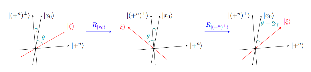
[Click the image for a larger version]
Clearly the angle \(\gamma\) remains fixed throughout, and we can calculate it exactly. Recall that states are of unit size and all of our amplitudes discussed are real numbers, so the angle \(\alpha\) between two states \(| x \rangle\), \(| y \rangle\) is given by the equation \(\cos \alpha = \langle y | x \rangle\). By inspecting the above diagram it then follows that
\[\sin \gamma = \cos \left(\frac{\pi}{2} - \gamma\right) = \langle +^n | x_0 \rangle = \frac{1}{\sqrt N}.\]Our system starts within the state \(| +^n \rangle\), so \(\theta = \frac{\pi}{2} - \gamma\). Let \(\theta_T\) denote the angle after T iterations and \(| \xi_T \rangle\) the corresponding state, then it follows quickly that \(\theta_T = \frac{\pi}{2} - (2T+1)\gamma\). We have that after T iterations, the probability of measuring \(x_0\) is precisely
\[\begin{align} |\langle \xi_T | x_0 \rangle |^2 &= \cos^2\theta_T \\ &= \cos^2 \left( \frac{\pi}{2} - (2T+1)\gamma \right) \\ &= \sin^2 \left( (2T+1)\gamma \right). \end{align}\]and our result follows. //
Corollary 2. The probability of measuring \(x_0\) is maximised when \(T \approx \frac \pi 4 \sqrt N\).
Proof. Clearly this probability is maximised when \((2T+1)\gamma\approx \frac{\pi}{2}\). To simplify the remaining calculations, we take the small-angle approximation \(\sin x \approx x\), so \(\gamma\) is approximately \(\frac{1}{\sqrt N}\). From here, it then follows that this probability is maximised when \(T \approx \frac{\pi}{4}\sqrt N\). //
This result demonstrates precisely our claim - that Grover’s algorithm finds the marked string with high probability, using just \(O (\sqrt N)\) queries.
5. Closing Remarks
This algorithm has been generalised and extended in several ways, to solve many different problems in the quantum realm. It generalises very nicely to the case of multiple marked elements, and Durr et al. [4] made use of a modified version of this to find the minimum element of a given list. Grover’s algorithm has been generalised even further to amplitude amplification and amplitude estimation [5], which boost the success of any arbitrary quantum algorithm and calculate the probability of success, respectively. These techniques can then be used in a variety of scenarios including fast mean-approximation [6].
It’s not hard to see then that this algorithm has had wide-reaching implications in the world of quantum computing, and the unstructured search problem is only the tip of the iceberg. The technology is still a long way behind the theory - quantum computers are not yet a viable tool at our disposal. However, despite the physical limitations, quantum algorithm theory is very much an active field of research and we can rest easy that when the first sufficiently powerful quantum computer presents itself, there will be no shortage of uses.
6. Bibliography
-
Grover, L.K., 1996. A fast quantum mechanical algorithm for database search. arXiv preprint quant-ph/9605043.
-
Montanaro, A., 2019. Quantum Computation lecture notes. Link.
-
Barnett, S.M., Introduction to Quantum Information. Link.
-
Durr, C. and Hoyer, P., 1996. A quantum algorithm for finding the minimum. arXiv preprint quant-ph/9607014.
-
Brassard, G., Hoyer, P., Mosca, M. and Tapp, A., 2002. Quantum amplitude amplification and estimation. Contemporary Mathematics, 305, pp.53-74.
-
Brassard, G., Dupuis, F., Gambs, S. and Tapp, A., 2011. An optimal quantum algorithm to approximate the mean and its application for approximating the median of a set of points over an arbitrary distance. arXiv preprint arXiv:1106.4267.